05 · Validation and measurement quality

Advanced notebook. In notebook 03 you calibrated real measurements and got a 75 Ω resistor to read about 74 Ω. Is that a good result? “It looks right” is not an answer you can put in a report. This notebook asks three questions of a measurement before trusting it, and then writes the answers down in a form someone else can check.

Learning objectives

After this notebook you will be able to:

• quantify the repeatability of a measurement from repeated sweeps, and turn it into a standard uncertainty;

• use passivity (\(|\Gamma| \le 1\)) as a physical test, and interpret a violation as evidence about the measurement;

• distinguish data integrity, physical consistency and measurement quality;

• record the context and processing history of a result so that it can be traced and reproduced.

You need: notebook 03. No hardware. This notebook uses one extra library, rfmeasurement.

import sys

if "google.colab" in sys.modules:
    %pip install -q "vnacourse[validation] @ git+https://github.com/telmomm/nanovna-measurement-course"

import matplotlib.pyplot as plt
import numpy as np
import skrf as rf
from IPython.display import Markdown
from rfmeasurement.domain import (
    AnalysisResult,
    Measurand,
    Measurement,
    MeasurementContext,
    MetadataConfidence,
    ProvenanceRecord,
    ValidationResult,
    ValidationStatus,
)
from rfmeasurement.reporting import generate_report
from rfmeasurement.validation import DEFAULT_RULES, PassivityRule, ValidationRule, validate

import vnacourse
from vnacourse import calibration, plotting
from vnacourse.data import load_repetitions
from vnacourse.reflection import gamma_to_z

plotting.use_course_style()

1. Three questions

Before using a measurement, ask:

1. Is the data intact? Right number of points, frequencies in order, no missing or infinite values. A failure here means the file is broken.

2. Is it physically plausible? A passive device cannot reflect more power than it receives. A failure here means the numbers contradict what we assumed about the device or the instrument.

3. How much does it change if I repeat it? That sets how many digits of the result mean anything.

These are different kinds of question, and the difference matters. A broken file must be thrown away. A physically implausible number must be explained: it is telling you something. We start with the third question, because its answer is needed to judge the second.

f_hz, short_reps = load_repetitions("standards", "short")
_, open_reps = load_repetitions("standards", "open")
_, load_reps = load_repetitions("standards", "load")
_, resistor_reps = load_repetitions("dut", "load_75ohm")
f_mhz = f_hz / 1e6

print(f"Standards: {open_reps.shape[0]} repetitions each, {len(f_hz)} frequency points")
print(f"75 Ω resistor: {resistor_reps.shape[0]} repetitions")

Standards: 10 repetitions each, 1001 frequency points
75 Ω resistor: 3 repetitions

2. Repeatability

Each standard was measured ten times without changing anything on purpose. If the instrument were perfectly repeatable the ten sweeps would be identical. They are not. At each frequency we summarise their scatter with a standard deviation. \(\Gamma\) is complex, so we combine the scatter of its real and imaginary parts:

\[s(f) = \sqrt{s^2_{\operatorname{Re}\Gamma}(f) + s^2_{\operatorname{Im}\Gamma}(f)}\]

Predict before you run. Which of the three standards do you expect to repeat best: the short, the open or the load? Think of what you learned about the error terms in notebook 02.

def spread(repetitions):
    """Standard deviation of a complex quantity across repetitions, per frequency."""
    return np.sqrt(repetitions.real.var(axis=0, ddof=1) + repetitions.imag.var(axis=0, ddof=1))


spreads = {"short": spread(short_reps), "open": spread(open_reps), "load": spread(load_reps)}

fig, ax = plt.subplots()
for name, s in spreads.items():
    ax.semilogy(f_mhz, s, label=name, linewidth=1.0)
    print(
        f"{name:<5} typical (median) {np.median(s):.4f}   mean {s.mean():.4f}   worst {s.max():.3f}"
    )
ax.set(xlabel="frequency (MHz)", ylabel="standard deviation of Γ (log scale)")
ax.set_title("Scatter of ten repetitions of each standard")
ax.legend(loc="upper center", bbox_to_anchor=(0.5, -0.18), ncol=3)

short typical (median) 0.0029   mean 0.0048   worst 0.060
open  typical (median) 0.0031   mean 0.0051   worst 0.069
load  typical (median) 0.0005   mean 0.0006   worst 0.004

<matplotlib.legend.Legend at 0x7fa0882b6ba0>

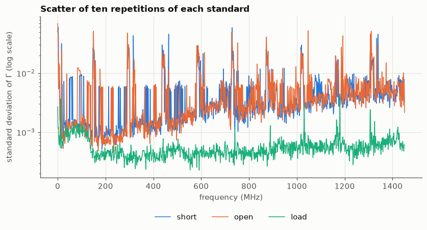
The load repeats about six times better than the short and the open. The reason is the one from notebook 02: anything that fluctuates in the return path multiplies \(\Gamma\), so it shows in full on a device with \(|\Gamma| = 1\) and hardly at all on one with \(\Gamma \approx 0\).

A typical scatter of 0.003 on a quantity of size 1 is 0.3 %. That number is the floor for everything else: no calibration computed from these sweeps can be trusted beyond it.

Look at the gap between the median and the mean, and at the worst value. The scatter is not uniform: there are spikes, twenty times above the typical level. Where are they?

s = spreads["open"]
noisy = np.flatnonzero(s > 5 * np.median(s))
print(f"{len(noisy)} of {len(s)} frequency points have more than 5 times the typical scatter")
print("Their positions in the sweep (index of the point):")
print(noisy)

just_after = np.sum(noisy % 100 < 10)
print(f"\n{just_after} of them fall in the first ten points after a multiple of 100")

53 of 1001 frequency points have more than 5 times the typical scatter
Their positions in the sweep (index of the point):
[  0   1  12 103 104 105 109 201 202 204 205 206 220 301 302 306 308 401
 403 405 406 407 408 409 423 502 503 504 505 519 601 602 604 607 702 704
 705 707 708 722 802 807 818 819 822 901 902 904 905 906 907 912 920]

43 of them fall in the first ten points after a multiple of 100

The noisy points are not spread at random. Most sit in the first few points after index 100, 200, 300 and so on, a tenth of the sweep. A device has no reason to be noisy at every hundredth point, so this pattern belongs to how the sweep was acquired, not to what was measured. It is what you would see if the instrument collected the 1001 points in blocks of about a hundred and needed a moment to settle at the start of each block. The data alone cannot confirm that explanation, but it does tell you where to look.

Two practical consequences:

• Use robust statistics to describe typical behaviour. The median is not pulled by a few spikes; the mean and the maximum are.

• A spike in one repetition contaminates the average of all ten. Exercise 1 compares averaging with taking the median across repetitions.

3. From repeatability to the uncertainty of a result

Take one concrete result: the resistance of the 75 Ω resistor below 10 MHz, defined as the mean of \(\operatorname{Re} Z\) over the points below 10 MHz, after SOL calibration. (Below 10 MHz the delay discussed in notebook 03 rotates the phase by only a few degrees, so we can read the resistance directly.)

Two things were repeated, so we have two sources of scatter:

• the resistor itself was measured 3 times;

• the calibration standards were measured 10 times, so we can compute 10 different calibrations.

For a mean of \(n\) repeated readings with standard deviation \(s\), the standard uncertainty of the mean is \(u = s/\sqrt{n}\). An uncertainty estimated this way, from statistics of repeated readings, is called Type A.

low = f_hz < 10e6


def resistance_below_10mhz(raw, terms):
    return gamma_to_z(calibration.correct(raw, terms)).real[low].mean()


all_standards = [reps.mean(axis=0) for reps in (short_reps, open_reps, load_reps)]
terms = calibration.solve_error_terms(all_standards)

# Source 1: the three repetitions of the resistor, each corrected with the full calibration.
r_per_sweep = np.array([resistance_below_10mhz(raw, terms) for raw in resistor_reps])

# Source 2: ten calibrations, one per repetition of the standards, applied to the mean sweep.
resistor_mean = resistor_reps.mean(axis=0)
r_per_calibration = np.array(
    [
        resistance_below_10mhz(
            resistor_mean,
            calibration.solve_error_terms([short_reps[i], open_reps[i], load_reps[i]]),
        )
        for i in range(len(open_reps))
    ]
)

u_dut = r_per_sweep.std(ddof=1) / np.sqrt(len(r_per_sweep))
u_cal = r_per_calibration.std(ddof=1) / np.sqrt(len(r_per_calibration))
u_combined = np.hypot(u_dut, u_cal)
resistance = resistance_below_10mhz(resistor_mean, terms)

print("Resistor sweeps:  ", np.round(r_per_sweep, 2), "Ω")
print("Calibrations:     ", np.round(r_per_calibration, 2), "Ω")
print(f"\nu from the resistor's repeatability:     {u_dut:.2f} Ω")
print(f"u from the calibration's repeatability:  {u_cal:.2f} Ω")
print(f"\nResistance below 10 MHz: {resistance:.1f} Ω, standard uncertainty {u_combined:.1f} Ω")

Resistor sweeps:   [73.93 73.74 74.31] Ω
Calibrations:      [73.92 74.05 73.95 74.09 73.58 74.03 74.07 74.35 73.9  73.98] Ω

u from the resistor's repeatability:     0.17 Ω
u from the calibration's repeatability:  0.06 Ω

Resistance below 10 MHz: 74.0 Ω, standard uncertainty 0.2 Ω

The two contributions are independent, so they combine as a root sum of squares. The result is about 74.0 Ω with a standard uncertainty of about 0.2 Ω.

The nominal value is 75 Ω: more than five standard uncertainties away. Repeatability cannot explain a difference that large, so something else is at work. The candidates are all things this uncertainty does not include:

• the resistor’s own tolerance (a common 1 % part may be anywhere from 74.25 Ω to 75.75 Ω, a 5 % part from 71 Ω to 79 Ω);

• the calibration standards, which we assumed ideal (notebook 03, section 6): an error there shifts every result in the same direction, every time, so repeating does not reveal it;

• whatever sits between the calibration plane and the resistor.

This is the most important habit of the notebook: an uncertainty is only meaningful together with the list of what it covers. “74.0 ± 0.2 Ω” on its own claims more than we know. “74.0 Ω, with 0.2 Ω of standard uncertainty from repeatability; standards assumed ideal” is honest.

4. Passivity as a physical test

A resistor, a short and an open are passive: they have no power source, so they cannot return more than they receive. For a one-port that means

\[|\Gamma| \le 1 \quad\text{at every frequency.}\]

This is a test that needs no reference device and no second measurement: the data either respects it or not. Apply it to three measurements:

• the raw open, as the instrument reported it;

• the open after calibration, using a calibration computed from repetitions 1–5 and applied to repetitions 6–10 (so the test is fair, as in notebook 03);

• the calibrated 75 Ω resistor.

Predict before you run. A perfect open has \(|\Gamma| = 1\) exactly. After a good calibration, with a little noise left, what fraction of the points do you expect to find above 1?

terms_first_half = calibration.solve_error_terms(
    [reps[:5].mean(axis=0) for reps in (short_reps, open_reps, load_reps)]
)

cases = {
    "open, raw": open_reps.mean(axis=0),
    "open, calibrated": calibration.correct(open_reps[5:].mean(axis=0), terms_first_half),
    "75 Ω resistor, calibrated": calibration.correct(resistor_mean, terms),
}

print(f"{'measurement':<27} {'largest |Γ|':>12} {'points above 1':>15} {'points above 1.01':>18}")
for name, gamma in cases.items():
    magnitude = np.abs(gamma)
    print(
        f"{name:<27} {magnitude.max():12.3f} {np.mean(magnitude > 1):15.0%} "
        f"{np.mean(magnitude > 1.01):18.1%}"
    )

measurement                  largest |Γ|  points above 1  points above 1.01
open, raw                          2.131             98%              24.5%
open, calibrated                   1.026             43%               0.3%
75 Ω resistor, calibrated          0.286              0%               0.0%

All three are different stories.

• The resistor is nowhere near the limit. Passivity holds.

• The raw open is above 1 at almost every point, and far above in a whole band. This is a real violation, and it is systematic: the same in all ten repetitions. It does not mean the file is corrupt. It means the instrument’s reflection tracking is not 1, which is exactly what notebook 02 predicted and what calibration then removed. The violation was evidence of an uncorrected systematic error.

• The calibrated open is above 1 at a little under half of the points, by tiny amounts. Look at how those amounts are distributed:

excess = np.abs(cases["open, calibrated"]) - 1

fig, ax = plt.subplots()
ax.hist(excess, bins=np.linspace(-0.012, 0.012, 49), color=plotting.SERIES[0])
ax.axvline(0, color=plotting.INK, linewidth=1.0)
ax.set(xlabel="$|\\Gamma| - 1$", ylabel="number of frequency points")
ax.set_title("Calibrated open: how far |Γ| is from 1")

inside = np.mean(np.abs(excess) < 0.012)
print(f"Median of |Γ| − 1: {np.median(excess):+.4f}")
print(f"Half of the points lie within ±{np.median(np.abs(excess)):.4f} of 1")
print(f"{1 - inside:.1%} of the points fall outside this plot")

Median of |Γ| − 1: -0.0001
Half of the points lie within ±0.0005 of 1
1.1% of the points fall outside this plot

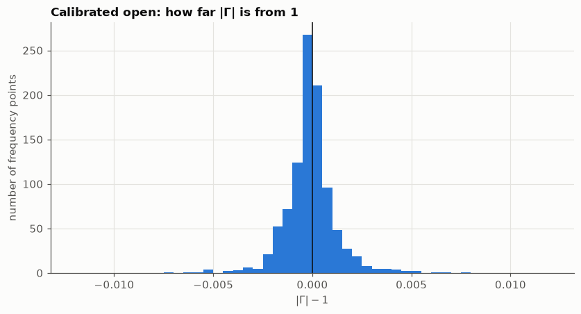
The values scatter on both sides of 1, in a narrow band: no wider than the repeatability from section 2 leads you to expect for a mean of five sweeps. This is what a device that reflects everything, measured with a little noise, must look like: noise does not know that 1 is a limit. A calibrated open with no point above 1 would be the suspicious result.

So “\(|\Gamma| > 1\)” has three possible meanings, and the size, the sign pattern and the repeatability tell them apart:

What you see	What it means	What to do
far above 1, in a band, the same in every repetition	uncorrected systematic error	calibrate (or check the calibration)
slightly above and below 1, comparable to the repeatability	noise around a fully reflecting device	nothing: report it with its uncertainty
isolated spikes	an acquisition problem at those points	look at how the sweep was taken

In none of them is the right response to discard the measurement or to clip the values to 1. Clipping would hide the evidence and bias the result. A passivity violation is an experimental finding, not a data error.

5. Writing the checks down: rfmeasurement

So far the checks live in your head and in scattered cells. rfmeasurement gives them a structure. Its ideas:

• a Measurement is the data (a scikit-rf Network) together with its context: instrument, calibration, device, and so on;

• a validation rule inspects a measurement and returns a result with a status (pass, warning, fail, not_applicable), the evidence it based the decision on, and an explanation;

• rules are grouped by the three questions of section 1: integrity.*, physics.* and quality.*.

The library ships a passivity rule, physics.passivity, written for networks with two or more ports; in version 0.3.0 it does not handle one-port data. We leave it out and write the one-port rule ourselves, which is also the best way to see what a rule is. Its tolerance comes from section 2: 0.01 is about three times the typical scatter of a fully reflecting standard.

class OnePortPassivityRule(ValidationRule):
    """|Γ| must not exceed 1 by more than the repeatability can explain."""

    identifier = "physics.passivity_one_port"
    description = "Reflection coefficient magnitude does not exceed 1."

    def __init__(self, tol=0.01, max_fraction=0.01):
        self.tol = tol
        self.max_fraction = max_fraction

    def is_applicable(self, measurement):
        return measurement.data.nports == 1

    def _evaluate(self, measurement):
        magnitude = np.abs(measurement.data.s[:, 0, 0])
        beyond = float(np.mean(magnitude > 1 + self.tol))
        evidence = {
            "max_magnitude": float(magnitude.max()),
            "fraction_above_1": float(np.mean(magnitude > 1)),
            "fraction_beyond_tolerance": beyond,
            "tolerance": self.tol,
        }
        if beyond > self.max_fraction:
            status = ValidationStatus.FAIL
            explanation = (
                "|Γ| exceeds 1 by more than the tolerance over a significant part of the band."
            )
        elif magnitude.max() > 1:
            status = ValidationStatus.WARNING
            explanation = (
                "|Γ| exceeds 1 only slightly or at isolated points: compare with repeatability."
            )
        else:
            status, explanation = ValidationStatus.PASS, None
        return ValidationResult(
            rule_id=self.identifier,
            status=status,
            description=self.description,
            evidence=evidence,
            explanation=explanation,
        )


rules = [rule for rule in DEFAULT_RULES if not isinstance(rule, PassivityRule)]
rules.append(OnePortPassivityRule())
print("Rules:", ", ".join(rule.identifier for rule in rules))

Rules: integrity.structural, integrity.finite_values, integrity.frequency_grid, physics.reciprocity, quality.continuity, quality.dynamic_range, physics.passivity_one_port

Wrap each of the three measurements of section 4 and validate it. The context says what we know about how each one was obtained.

frequency = rf.Frequency.from_f(f_hz, unit="Hz")
calibrations = {
    "open, raw": "none (raw)",
    "open, calibrated": "SOL, ideal standards, repetitions 1-5",
    "75 Ω resistor, calibrated": "SOL, ideal standards, repetitions 1-10",
}

measurements = {}
for name, gamma in cases.items():
    measurement = Measurement(
        data=rf.Network(frequency=frequency, s=gamma, z0=50, name=name),
        context=MeasurementContext(
            dut=name.split(",")[0],
            instrument="NanoVNA-F V2",
            calibration=calibrations[name],
            frequency_range_hz=(float(f_hz[0]), float(f_hz[-1])),
        ),
    )
    measurement.validation = validate(measurement, rules)
    measurements[name] = measurement

print(f"{'rule':<28}" + "".join(f"{name:>28}" for name in measurements))
for i, rule in enumerate(rules):
    statuses = [m.validation.results[i].status.value for m in measurements.values()]
    print(f"{rule.identifier:<28}" + "".join(f"{status:>28}" for status in statuses))

rule                                           open, raw            open, calibrated   75 Ω resistor, calibrated
integrity.structural                                pass                        pass                        pass
integrity.finite_values                             pass                        pass                        pass
integrity.frequency_grid                            pass                        pass                        pass
physics.reciprocity                       not_applicable              not_applicable              not_applicable
quality.continuity                                  pass                        pass                        pass
quality.dynamic_range                               pass                        pass                        pass
physics.passivity_one_port                          fail                     warning                        pass

Read the table by rows. The three integrity rules pass everywhere: the files are fine. Reciprocity does not apply to a one-port. The quality rules pass. Only the physics row differs: fail for the raw open, warning for the calibrated open, pass for the resistor. Those are the three stories of section 4, now as a record.

A status alone would be a traffic light. What makes it useful is the evidence that comes with it:

for name, measurement in measurements.items():
    result = measurement.validation.results[-1]
    print(f"{name}: {result.status.value}")
    for key, value in result.evidence.items():
        print(f"    {key}: {value:.4g}")
    if result.explanation:
        print(f"    {result.explanation}")

open, raw: fail
    max_magnitude: 2.131
    fraction_above_1: 0.984
    fraction_beyond_tolerance: 0.2448
    tolerance: 0.01
    |Γ| exceeds 1 by more than the tolerance over a significant part of the band.
open, calibrated: warning
    max_magnitude: 1.026
    fraction_above_1: 0.4326
    fraction_beyond_tolerance: 0.002997
    tolerance: 0.01
    |Γ| exceeds 1 only slightly or at isolated points: compare with repeatability.
75 Ω resistor, calibrated: pass
    max_magnitude: 0.2859
    fraction_above_1: 0
    fraction_beyond_tolerance: 0
    tolerance: 0.01

6. Traceability: what would someone else need?

Suppose a colleague reads “the resistor is 74.0 Ω” a year from now. To trust it or to redo it, they need to know which instrument, which calibration, which data, which processing steps and which software. That is traceability, and it is cheap to record at the time and impossible to reconstruct afterwards.

The context of a measurement has a field for each thing worth knowing. Print it for our resistor and see how much is missing:

resistor = measurements["75 Ω resistor, calibrated"]
resistor.context.averaging = len(resistor_reps)
resistor.context.confidence = {
    "instrument": MetadataConfidence.SPECIFIED,
    "calibration": MetadataConfidence.ASSUMED,
    "frequency_range_hz": MetadataConfidence.MEASURED,
}

for field in resistor.context.__dataclass_fields__:
    value = getattr(resistor.context, field)
    if field == "confidence":
        value = {key: level.value for key, level in value.items()}
    known = value is not None and value != {}
    print(f"{field:<20} {value if known else '— unknown'}")

dut                  75 Ω resistor
operator             — unknown
instrument           NanoVNA-F V2
calibration          SOL, ideal standards, repetitions 1-10
cables               — unknown
fixture              — unknown
temperature_c        — unknown
humidity_percent     — unknown
pressure_pa          — unknown
rf_power_dbm         — unknown
if_bandwidth_hz      — unknown
averaging            3
sweep_settings       — unknown
frequency_range_hz   (50000.0, 1450000000.0)
timestamp            — unknown
confidence           {'instrument': 'specified', 'calibration': 'assumed', 'frequency_range_hz': 'measured'}

Operator, cables, fixture, temperature, power, bandwidth, date: all unknown. That is not a criticism of this dataset in particular; it is what almost every measurement file looks like a few months later. Note the confidence entry too: the instrument is specified (we were told), the frequency range is measured (it is in the data), and the calibration is assumed (ideal standards). An honest record separates what was measured from what was taken on trust.

The other half of traceability is the processing history: each step that turned raw sweeps into the reported number. Record the steps, then ask rfmeasurement for a report of the result from section 3.

software = f"vnacourse {vnacourse.__version__}"
averaged = ProvenanceRecord(
    operation="average repetitions",
    software_version=software,
    parameters={"repetitions": len(resistor_reps)},
    inputs=("data/dut/load_75ohm",),
)
calibrated = ProvenanceRecord(
    operation="SOL calibration",
    software_version=software,
    parameters={"standards": "assumed ideal", "repetitions_averaged": len(open_reps)},
    inputs=(averaged.record_id, "data/standards"),
)
resistor.provenance = [averaged, calibrated]

report = resistor.validation
if report.has_failures:
    overall = ValidationStatus.FAIL
elif report.has_warnings:
    overall = ValidationStatus.WARNING
else:
    overall = ValidationStatus.PASS

result = AnalysisResult(
    measurand=Measurand(
        name="Resistance below 10 MHz",
        definition="mean of Re Z over the frequency points below 10 MHz",
        unit="ohm",
    ),
    value=round(float(resistance), 2),
    unit="ohm",
    standard_uncertainty=round(float(u_combined), 2),
    provenance=(averaged, calibrated),
    validation_status=overall,
)

Markdown(generate_report(resistor, result))

Analysis report: Resistance below 10 MHz

Result

• value: 73.99 ohm

• standard uncertainty: 0.18 ohm

• validation status at analysis time: pass

Input

• network: 75 Ω resistor, calibrated

• ports: 1

• frequency range: 50000-1.45e+09 Hz

Validation summary

Overall: OK (warnings=False)

• [PASS] integrity.structural: S-parameter array shape is consistent with the frequency grid and port count.

• [PASS] integrity.finite_values: All S-parameter samples are finite.

• [PASS] integrity.frequency_grid: Frequency points are strictly increasing with no duplicates.

• [NOT_APPLICABLE] physics.reciprocity: Network is reciprocal (S equals its transpose).

• [PASS] quality.continuity: No S-parameter magnitude jump between adjacent frequency points exceeds the threshold.

• [PASS] quality.dynamic_range: Smallest observed S-parameter magnitude is above the configured noise-floor margin.

• [PASS] physics.passivity_one_port: Reflection coefficient magnitude does not exceed 1.

Analysis configuration

• validation rules evaluated: integrity.structural, integrity.finite_values, integrity.frequency_grid, physics.reciprocity, quality.continuity, quality.dynamic_range, physics.passivity_one_port

Software environment

• rfmeasurement: 0.3.0

• Python: 3.12.14

• numpy: 2.5.3

• scikit-rf: 2.1.0

• scipy: 1.18.1

Reproducibility level

Level 4: Level 3 plus complete instrument/calibration/environment provenance.

See docs/reproducibility.md for the full level definitions.

One page holds the value, its uncertainty, which checks were run and how they came out, the software versions, and a reproducibility level. The level reported is the highest one because we supplied the instrument, the calibration and a processing history. It does not judge whether those are good: an assumed-ideal calibration counts as recorded. The report makes the record complete; the judgement in sections 3 and 4 is still yours.

Check your understanding

1. Ten repetitions give a standard deviation of 0.003. What is the standard uncertainty of their mean? How many repetitions would you need to halve it?

Answer

\(u = 0.003/\sqrt{10} \approx 0.001\). Uncertainty falls as \(1/\sqrt{n}\), so halving it takes four times as many: 40 repetitions.

2. Averaging more repetitions reduces the 0.2 Ω uncertainty of section 3. Does it bring the result closer to the true resistance?

Answer

Only as far as random error is concerned. If the load standard is not exactly 50 Ω, every calibration is wrong in the same way and the average converges, ever more precisely, to the wrong value. Repetition reduces random error; it does nothing about systematic error.

3. A colleague suggests cleaning the data by replacing every \(|\Gamma| > 1\) with exactly 1. What is wrong with that?

Answer

For the calibrated open, noise scatters on both sides of 1. Clipping only the upper side pulls the average below 1: it introduces a bias. It also destroys the evidence: afterwards nobody can tell whether the excursions were noise, an acquisition spike or a calibration problem.

4. Which validation status would you assign to a file in which two frequency points are in the wrong order: integrity, physics or quality? Would you treat it like the passivity failure of the raw open?

Answer

Integrity. It is a different kind of failure: the data structure itself is wrong, so nothing computed from it can be trusted until it is fixed. A physics failure on an intact file is a finding about the measurement and should be kept and explained.

Exercises

Worked solutions are in exercises/solutions/05_solutions.ipynb.

1. Mean or median? Recompute the calibration of section 4 (repetitions 1–5) using the median across repetitions instead of the mean (take the median of the real and imaginary parts separately). Correct the mean and the median of repetitions 6–10 of the open and compare the worst-case and the typical distance from \(\Gamma = 1\). Which statistic handles the spikes better?

2. Uncertainty across the band. Section 3 looked only below 10 MHz. Compute the spread of the calibrated \(\Gamma\) of the 75 Ω resistor across the ten single-repetition calibrations at every frequency, and plot it. Is the calibration equally repeatable over the whole band?

3. Write a rule. Write a ValidationRule called quality.spikes that warns when a single sweep has points that differ from the median of their neighbours by more than a threshold. Apply it to one repetition of the raw open and report where the spikes are.

4. Your own context. Fill in a MeasurementContext for a measurement you could take in your laboratory. For each field decide whether its value would be measured, specified, estimated or assumed.

# Your work here

Summary

• Repeated sweeps give the repeatability of a measurement. Here it is about 0.003 for fully reflecting devices and 0.0005 for a matched one, with spikes tied to the acquisition.

• The standard uncertainty of a mean of \(n\) readings is \(s/\sqrt{n}\). It covers random error only; say what it leaves out.

• Passivity, \(|\Gamma| \le 1\), is a physical test that needs no reference. A violation is evidence: of a systematic error if it is large and repeatable, of noise if it is as small as the repeatability.

• Integrity, physical consistency and quality are different questions with different consequences.

• A result is traceable when its context and processing history are recorded with it.

This is the last notebook of the core module. Notebook 04, on acquiring your own measurements with a NanoVNA, is optional, needs the instrument, and is not yet available.