

Solutions · 03 SOL calibration#
Worked solutions to the exercises of notebook 03. Try each exercise yourself first.
import sys

if "google.colab" in sys.modules:
    %pip install -q git+https://github.com/telmomm/nanovna-measurement-course
import matplotlib.pyplot as plt
import numpy as np

from vnacourse import plotting
from vnacourse.calibration import correct, solve_error_terms
from vnacourse.data import load_repetitions
from vnacourse.errormodel import ErrorTerms, apply_error_model, synthetic_error_terms
from vnacourse.reflection import gamma_to_z, z_to_gamma

plotting.use_course_style()

f_real, short_reps = load_repetitions("standards", "short")
_, open_reps = load_repetitions("standards", "open")
_, load_reps = load_repetitions("standards", "load")
f_real_mhz = f_real / 1e6
standards = (short_reps, open_reps, load_reps)
ideal = [-1.0, 1.0, 0.0]

f_hz = np.linspace(50e3, 1.45e9, 401)
ones = np.ones(f_hz.shape)
true_terms = synthetic_error_terms(f_hz)
1. Closed form#
Call the raw readings of the short, open and load \(s\), \(o\) and \(l\), and write \(t = e_{10}e_{01}\). The model \(\Gamma_m = e_{00} + t\,\Gamma/(1 - e_{11}\Gamma)\) gives:
load, \(\Gamma = 0\): \(\; l = e_{00}\)
open, \(\Gamma = +1\): \(\; (o - e_{00})(1 - e_{11}) = t\)
short, \(\Gamma = -1\): \(\; (s - e_{00})(1 + e_{11}) = -t\)
Adding the last two eliminates \(t\):
def solve_closed_form(short, open_, load):
    e00 = load
    e11 = (open_ + short - 2 * e00) / (open_ - short)
    tracking = (open_ - e00) * (1 - e11)
    return ErrorTerms(e00, e11, tracking)


measured = [reps.mean(axis=0) for reps in standards]
by_hand = solve_closed_form(*measured)
by_solver = solve_error_terms(measured, ideal)

for name, a, b in zip(ErrorTerms._fields, by_hand, by_solver, strict=True):
    print(f"{name:<13} largest difference: {np.abs(a - b).max():.1e}")
directivity   largest difference: 1.2e-16
source_match  largest difference: 5.7e-16
tracking      largest difference: 6.7e-16
The same terms, to rounding error, with no matrix. The closed form also shows what each standard is for: the load gives the directivity directly, and the short and the open, being opposite, separate the source match (their sum) from the tracking (their difference). It only works for ideal standards; the matrix form accepts any known \(\Gamma\).
2. Fewer repetitions#
Calibrate with the mean of repetitions 1–5 and with repetition 1 alone, and test both on the mean of repetitions 6–10.
test = [reps[5:].mean(axis=0) for reps in standards]
calibrations = {
    "five repetitions": [reps[:5].mean(axis=0) for reps in standards],
    "one repetition": [reps[0] for reps in standards],
}

for label, train in calibrations.items():
    terms = solve_error_terms(train, ideal)
    print(label)
    for name, raw, target in zip(("short", "open", "load"), test, ideal, strict=True):
        residual = np.abs(correct(raw, terms) - target)
        print(f"   {name:<5} median {np.median(residual):.4f}   worst {residual.max():.3f}")
five repetitions
   short median 0.0015   worst 0.045
   open  median 0.0016   worst 0.040
   load  median 0.0003   worst 0.003
one repetition
   short median 0.0024   worst 0.089
   open  median 0.0023   worst 0.054
   load  median 0.0005   worst 0.005
With a single repetition the typical residual grows by a factor of about 1.6, and the worst case roughly doubles for the short.
Why 1.6 and not \(\sqrt{5} \approx 2.2\)? The residual contains the noise of the calibration and the noise of the test data, which is a mean of five in both cases. If one sweep has noise \(\sigma\), the two cases compare as \(\sqrt{\sigma^2 + \sigma^2/5}\) against \(\sqrt{\sigma^2/5 + \sigma^2/5}\), a ratio of \(\sqrt{3} \approx 1.7\). Close to what we see.
Averaging is cheap and it pays, but with diminishing returns: each halving of the noise costs four times as many sweeps.
3. Two parametrisations#
terms = solve_error_terms(measured, ideal)
ed, es = terms.directivity, terms.source_match
er = terms.tracking - ed * es

difference = np.abs(er - terms.tracking)
fig, ax = plt.subplots()
ax.semilogy(f_real_mhz, difference)
ax.set(xlabel="frequency (MHz)", ylabel="$|e_r - e_{10}e_{01}|$ (log scale)")
ax.set_title("Difference between the two definitions of the third term")

worst = difference.argmax()
print(f"Largest difference: {difference.max():.4f} at {f_real_mhz[worst]:.0f} MHz")
print(f"Largest difference above 150 MHz: {difference[f_real > 150e6].max():.1e}")

_, resistor = load_repetitions("dut", "load_75ohm")
raw = resistor.mean(axis=0)
other_form = (raw - ed) / (er + es * raw)
print("Same corrected Γ with both forms:", np.allclose(other_form, correct(raw, terms)))
Largest difference: 0.0022 at 64 MHz
Largest difference above 150 MHz: 2.1e-05
Same corrected Γ with both forms: True
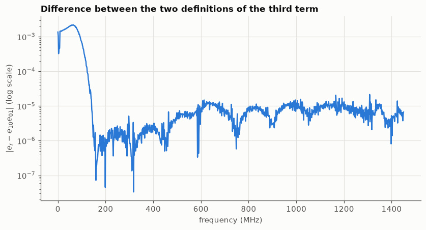
The two quantities differ by exactly \(e_{00}e_{11}\), the product of directivity and source match. That product is largest (about 0.002) near 64 MHz, in the band where both terms are large, and negligible above 150 MHz where both are small.
The corrected \(\Gamma\) is identical, because both expressions are the same formula written with different unknowns:
So the choice does not affect any result. It matters only when you interpret or compare the terms: \(e_r\) is not, strictly, the reflection tracking. For this instrument the difference is at most 0.2 %.
4. A fourth standard#
With four standards the system has four equations and three unknowns, and np.linalg.lstsq finds the terms that fit all four best. To see whether that helps we need noise: without it both solutions are exact. We add noise of standard deviation 0.003 (the repeatability measured in notebook 05) to the “measurements” of the standards, calibrate, correct a noise-free 33 Ω device, and repeat many times.
def solve_least_squares(measured, actual):
    """Like solve_error_terms, for three or more standards."""
    actual = np.asarray(actual, dtype=complex)
    solution = np.empty((len(f_hz), 3), dtype=complex)
    for k in range(len(f_hz)):
        m = np.array([standard[k] for standard in measured])
        matrix = np.column_stack([np.ones(len(m)), actual * m, -actual])
        solution[k], *_ = np.linalg.lstsq(matrix, m, rcond=None)
    e00, e11, delta = solution.T
    return ErrorTerms(e00, e11, e00 * e11 - delta)


rng = np.random.default_rng(0)
noise_level = 0.003
known = [-1.0, 1.0, 0.0, float(z_to_gamma(75).real)]  # short, open, load, 75 Ω
device = z_to_gamma(33) * ones
device_raw = apply_error_model(device, true_terms)

errors = {3: [], 4: []}
for _ in range(200):
    noisy = [
        apply_error_model(gamma * ones, true_terms)
        + noise_level
        * (rng.standard_normal(f_hz.shape) + 1j * rng.standard_normal(f_hz.shape))
        / np.sqrt(2)
        for gamma in known
    ]
    for n in errors:
        terms_n = solve_least_squares(noisy[:n], known[:n])
        errors[n].append(np.abs(correct(device_raw, terms_n) - device))

for n, values in errors.items():
    print(
        f"{n} standards: RMS error of the corrected Γ = {np.sqrt(np.mean(np.square(values))):.4f}"
    )
3 standards: RMS error of the corrected Γ = 0.0033
4 standards: RMS error of the corrected Γ = 0.0025
The fourth standard reduces the error of the corrected device by about a quarter. The extra equation lets the noise of the individual standards partly average out, and a standard inside the chart constrains the calibration where the short and the open, both on the rim, do not.
Two remarks. The gain depends on where the device is: it is largest for devices in the middle of the chart and small for devices near the rim (try a device with \(\Gamma = 0.8\)). And in practice the bigger benefit of a fourth standard is not noise: with three standards the fit is always perfect, so you learn nothing about its quality; with four, the residual of the fit tells you whether your standards are consistent with each other.
5. How much does the open matter?#
Repeat section 6 for three values of the fringing capacitance. To see the effect of the open alone we also run it with a perfect short and load.
omega = 2 * np.pi * f_hz
device_raw = apply_error_model(z_to_gamma(75) * ones, true_terms)

print(
    f"{'C of the open':>14} {'Z at 1.45 GHz, only the open imperfect':>40} {'as in section 6':>24}"
)
for capacitance in (0.05e-12, 0.1e-12, 0.2e-12):
    real_open = z_to_gamma(1 / (1j * omega * capacitance))
    row = []
    for real_short, real_load in (
        (-ones, 0 * ones),
        (z_to_gamma(1j * omega * 0.3e-9), z_to_gamma(51.5) * ones),
    ):
        seen = [apply_error_model(g, true_terms) for g in (real_short, real_open, real_load)]
        terms_ideal = solve_error_terms(seen, ideal)
        row.append(gamma_to_z(correct(device_raw, terms_ideal))[-1])
    print(f"{capacitance * 1e12:11.2f} pF {row[0]:>32.1f} Ω {row[1]:>22.1f} Ω")
 C of the open   Z at 1.45 GHz, only the open imperfect          as in section 6
       0.05 pF                        75.0+0.9j Ω              72.7+2.0j Ω
       0.10 pF                        74.9+1.7j Ω              72.6+2.8j Ω
       0.20 pF                        74.5+3.4j Ω              72.3+4.3j Ω
With only the open imperfect, the 75 Ω resistor picks up a false reactance of about 0.9 Ω, 1.7 Ω and 3.4 Ω at 1.45 GHz: proportional to the capacitance we ignored, while the resistance hardly moves. An unmodelled capacitance in the open shows up as a reactance error in everything measured afterwards.
With the imperfect short and load of section 6 as well, the errors add: the resistance is about 2.3 Ω low (the load) and the reactance error grows further (the short’s inductance pushes the same way).
For scale: capacitances of this order, tens to a couple of hundred femtofarads, are what an open coaxial connector has. At 1.45 GHz that is already a 1 % to 5 % error on a 75 Ω device, and it grows in proportion to frequency. This is why calibration kits ship with a definition of each standard.