Solutions · 01 Reflection coefficient and the Smith chart

Worked solutions to the exercises of notebook 01. Try each exercise yourself first, especially the mystery circuits.

import sys

if "google.colab" in sys.modules:
    %pip install -q git+https://github.com/telmomm/nanovna-measurement-course

import matplotlib.pyplot as plt
import numpy as np

from vnacourse import plotting
from vnacourse.puzzles import mystery_trace
from vnacourse.reflection import gamma_to_z, z_to_gamma

plotting.use_course_style()

Z0 = 50.0
f_hz = np.linspace(10e6, 1.45e9, 600)
omega = 2 * np.pi * f_hz

1. There and back

By hand, for \(Z = 20 - j30\ \Omega\):

\[\Gamma = \frac{(20 - j30) - 50}{(20 - j30) + 50} = \frac{-30 - j30}{70 - j30} = \frac{(-30 - j30)(70 + j30)}{70^2 + 30^2} = \frac{-1200 - j3000}{5800} = -0.207 - j0.517\]

gamma = z_to_gamma(20 - 30j)
print(f"Γ = {gamma:.3f},  |Γ| = {abs(gamma):.3f},  angle = {np.degrees(np.angle(gamma)):.1f}°")
print(f"Back to impedance: {gamma_to_z(gamma):.1f} Ω")

gamma_2 = 0.5 * np.exp(1j * np.radians(90))
print(f"\nΓ = 0.5∠90°  →  Z = {gamma_to_z(gamma_2):.1f} Ω")

Γ = -0.207-0.517j,  |Γ| = 0.557,  angle = -111.8°
Back to impedance: 20.0-30.0j Ω

Γ = 0.5∠90°  →  Z = 30.0+40.0j Ω

The point is in the lower-left of the chart: resistance below 50 Ω (left) and capacitive (lower half). The second point, \(\Gamma = j0.5\), is \(Z = 30 + j40\ \Omega\): straight above the centre does not mean 50 Ω of resistance. The 50 Ω circle passes through the centre but bends to the right.

2. Admittance

Take any impedances \(Z\) and compare \(\Gamma(Z)\) with \(\Gamma(Z_0^2/Z)\).

rng = np.random.default_rng(1)
z = rng.uniform(1, 300, 5) + 1j * rng.uniform(-300, 300, 5)

for z_k in z:
    mirrored = z_to_gamma(Z0**2 / z_k)
    print(f"Z = {z_k:7.1f} Ω   Γ(Z) = {z_to_gamma(z_k):+.3f}   Γ(Z0²/Z) = {mirrored:+.3f}")

assert np.allclose(z_to_gamma(Z0**2 / z), -z_to_gamma(z))

Z = 154.0-46.0j Ω   Γ(Z) = +0.534-0.105j   Γ(Z0²/Z) = -0.534+0.105j
Z = 285.2+196.6j Ω   Γ(Z) = +0.778+0.130j   Γ(Z0²/Z) = -0.778-0.130j
Z = 44.1-54.5j Ω   Γ(Z) = +0.204-0.461j   Γ(Z0²/Z) = -0.204+0.461j
Z = 284.6+29.8j Ω   Γ(Z) = +0.704+0.026j   Γ(Z0²/Z) = -0.704-0.026j
Z = 94.2-283.5j Ω   Γ(Z) = +0.857-0.280j   Γ(Z0²/Z) = -0.857+0.280j

Always opposite. Algebraically, with \(Z' = Z_0^2/Z\):

\[\Gamma' = \frac{Z_0^2/Z - Z_0}{Z_0^2/Z + Z_0} = \frac{Z_0 - Z}{Z_0 + Z} = -\Gamma\]

The normalised impedance of \(Z'\) is \(Z'/Z_0 = Z_0/Z\), which is the normalised admittance of \(Z\). So rotating a point by 180° around the centre turns “reading impedance” into “reading admittance”. A line of constant conductance is therefore the image, under that rotation, of a line of constant resistance: the conductance circles are the resistance circles mirrored through the centre, touching the short instead of the open.

3. Parallel resonance

\(\dfrac{1}{Z} = \dfrac{1}{R} + \dfrac{1}{j\omega L} + j\omega C\), with resonance again at \(f_0 = 1/(2\pi\sqrt{LC})\).

R, L, C = 100.0, 5e-9, 20e-12
z_parallel = 1 / (1 / R + 1 / (1j * omega * L) + 1j * omega * C)
f0 = 1 / (2 * np.pi * np.sqrt(L * C))
gamma = z_to_gamma(z_parallel)

fig, ax = plt.subplots(figsize=(5.4, 5.4))
plotting.gamma_plane(ax, title="Parallel RLC: 100 Ω ∥ 5 nH ∥ 20 pF")
ax.plot(gamma.real, gamma.imag, label="trace, 10 MHz to 1.45 GHz")
ax.plot(gamma[0].real, gamma[0].imag, "o", color=plotting.SERIES[0])
ax.plot(z_to_gamma(R).real, 0, "s", color=plotting.INK)
ax.annotate("$f_0$", (z_to_gamma(R).real, 0), xytext=(8, 8), textcoords="offset points")
ax.legend(loc="upper left", bbox_to_anchor=(0.0, 0.0))

below = f_hz < f0
print(f"Resonant frequency: {f0 / 1e6:.0f} MHz")
print(f"Reactance below resonance is positive (inductive): {np.all(z_parallel.imag[below] > 0)}")
print(f"Reactance above resonance is negative (capacitive): {np.all(z_parallel.imag[~below] < 0)}")

Resonant frequency: 503 MHz
Reactance below resonance is positive (inductive): True
Reactance above resonance is negative (capacitive): True

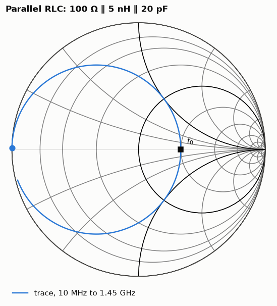
At resonance the inductor and the capacitor cancel as admittances and only the resistor is left: the trace crosses the horizontal axis at the 100 Ω point. The trace follows the 100 Ω conductance circle.

Below resonance the circuit is inductive (upper half) and above it is capacitive: the opposite of the series circuit. In parallel, the element with the smaller impedance dominates, and at low frequency that is the inductor. The trace still turns clockwise.

4. The mystery circuits

The method is the same for the three: look at the shape to decide the topology, then read the values from the impedance (series) or the admittance (parallel).

Circuit A

The trace starts near the open, stays in the lower half and follows a resistance circle: a resistor in series with a capacitor. Then \(\operatorname{Re} Z = R\) and \(\operatorname{Im} Z = -1/(\omega C)\).

z_a = gamma_to_z(mystery_trace("A", f_hz))
r_a = z_a.real
c_a = -1 / (omega * z_a.imag)
print(f"Re Z: {r_a.min():.2f} to {r_a.max():.2f} Ω  →  R = {r_a.mean():.0f} Ω")
print(f"C from every frequency point: {c_a.min() * 1e12:.2f} to {c_a.max() * 1e12:.2f} pF")

Re Z: 30.00 to 30.00 Ω  →  R = 30 Ω
C from every frequency point: 8.00 to 8.00 pF

A is 30 Ω in series with 8 pF. That \(R\) and \(C\) come out the same at every frequency confirms the topology: with the wrong model they would drift.

Circuit B

The trace starts at the short, rises through the upper half along a circle that touches the short, and heads for a point on the right of the horizontal axis: a resistor in parallel with an inductor. Work with the admittance \(Y = 1/Z = 1/R + 1/(j\omega L)\).

y_b = 1 / gamma_to_z(mystery_trace("B", f_hz))
r_b = 1 / y_b.real
l_b = -1 / (omega * y_b.imag)
print(f"1 / Re Y: {r_b.min():.1f} to {r_b.max():.1f} Ω  →  R = {r_b.mean():.0f} Ω")
print(f"L from every frequency point: {l_b.min() * 1e9:.2f} to {l_b.max() * 1e9:.2f} nH")

1 / Re Y: 120.0 to 120.0 Ω  →  R = 120 Ω
L from every frequency point: 15.00 to 15.00 nH

B is 120 Ω in parallel with 15 nH.

Circuit C

The trace follows a resistance circle from the lower half to the upper half and crosses the horizontal axis: a series RLC. The resistance is \(\operatorname{Re} Z\), the resonant frequency is where \(\operatorname{Im} Z = 0\), and the reactance \(X = \omega L - \dfrac{1}{\omega C}\) is linear in the two unknowns \(L\) and \(1/C\), so a least-squares fit over all frequencies gives both.

z_c = gamma_to_z(mystery_trace("C", f_hz))
r_c = z_c.real.mean()

crossing = np.flatnonzero(np.diff(np.sign(z_c.imag)))[0]
f0_c = np.interp(0, z_c.imag[crossing : crossing + 2], f_hz[crossing : crossing + 2])

# Scale the two columns to similar sizes (ω is ~1e9, 1/ω is ~1e-10) so the fit is well conditioned.
omega_ref = 2 * np.pi * 1e9
design = np.column_stack([omega / omega_ref, -omega_ref / omega])
(a, b), *_ = np.linalg.lstsq(design, z_c.imag, rcond=None)
l_c, inverse_c = a / omega_ref, b * omega_ref

print(f"R = {r_c:.0f} Ω")
print(f"Resonance (Im Z = 0) at {f0_c / 1e6:.0f} MHz")
print(f"L = {l_c * 1e9:.1f} nH,  C = {1 / inverse_c * 1e12:.2f} pF")
print(f"Check: 1 / (2π√(LC)) = {1 / (2 * np.pi * np.sqrt(l_c / inverse_c)) / 1e6:.0f} MHz")

R = 60 Ω
Resonance (Im Z = 0) at 650 MHz
L = 30.0 nH,  C = 2.00 pF
Check: 1 / (2π√(LC)) = 650 MHz

C is 60 Ω in series with 30 nH and 2 pF, resonant at 650 MHz.

Knowing \(f_0\) alone would give only the product \(LC\). The second piece of information is how fast the reactance changes around resonance, which is what the fit uses. With real, noisy data you would do the same, and the residual of the fit would tell you how well the three-element model describes the device.