03 · SOL calibration

In notebook 02 you saw that an instrument distorts every reflection through three error terms. Calibration is how you find those three terms and undo them. On the instrument it is a menu: connect the short, press a button; connect the open, press a button; connect the load, press a button. Here you do what happens behind those buttons.

Learning objectives

After this notebook you will be able to:

• turn the three-term error model into a system of three linear equations and solve it;

• correct a raw measurement with the error terms you found;

• check a calibration against data that was not used to compute it;

• explain what a calibration does not fix: the reference plane and imperfect standards.

You need: the three-term error model from notebook 02. No hardware: the real measurements are included.

import sys

if "google.colab" in sys.modules:
    %pip install -q git+https://github.com/telmomm/nanovna-measurement-course

import matplotlib.pyplot as plt
import numpy as np
import skrf as rf

from vnacourse import plotting
from vnacourse.data import load_repetitions
from vnacourse.errormodel import ErrorTerms, apply_error_model, synthetic_error_terms
from vnacourse.reflection import gamma_to_z, z_to_gamma

plotting.use_course_style()

1. Three unknowns, three equations

The error model, at one frequency, is

\[\Gamma_m = e_{00} + \frac{e_{10}e_{01}\,\Gamma}{1 - e_{11}\,\Gamma}\]

It has three unknown complex numbers. If you measure a device whose true \(\Gamma\) you already know, you get one equation. Three known devices, called calibration standards, give three equations. The usual choice is a Short (\(\Gamma = -1\)), an Open (\(\Gamma = +1\)) and a Load (\(\Gamma = 0\)): three points as far apart as possible on the \(\Gamma\) plane.

The equation is not linear in the error terms as written, because \(e_{11}\) sits in a denominator. Multiply both sides by \((1 - e_{11}\Gamma)\) and group:

\[\Gamma_m = e_{00} + \Gamma\,\Gamma_m\,e_{11} - \Gamma\,\Delta_e \qquad\text{with}\qquad \Delta_e = e_{00}e_{11} - e_{10}e_{01}\]

Now it is linear in the three unknowns \(e_{00}\), \(e_{11}\) and \(\Delta_e\). Writing it once per standard:

\[\begin{split} \begin{bmatrix} 1 & \Gamma_1\Gamma_{m1} & -\Gamma_1 \\ 1 & \Gamma_2\Gamma_{m2} & -\Gamma_2 \\ 1 & \Gamma_3\Gamma_{m3} & -\Gamma_3 \end{bmatrix} \begin{bmatrix} e_{00} \\ e_{11} \\ \Delta_e \end{bmatrix} = \begin{bmatrix} \Gamma_{m1} \\ \Gamma_{m2} \\ \Gamma_{m3} \end{bmatrix} \end{split}\]

Solve this 3×3 system at every frequency, then recover the tracking as \(e_{10}e_{01} = e_{00}e_{11} - \Delta_e\).

Correction. Once the terms are known, solve the model for \(\Gamma\):

\[\Gamma = \frac{\Gamma_m - e_{00}}{e_{10}e_{01} + e_{11}\,(\Gamma_m - e_{00})}\]

Read it from the inside out: subtract the directivity, then undo tracking and source match together.

2. Write the solver

measured and actual each hold three arrays (one per standard), with one value per frequency. The loop builds and solves the 3×3 system frequency by frequency.

def solve_error_terms(measured, actual):
    """Error terms from three standards: what was measured and what they really are."""
    n_freq = len(measured[0])
    e00 = np.empty(n_freq, dtype=complex)
    e11 = np.empty(n_freq, dtype=complex)
    delta = np.empty(n_freq, dtype=complex)
    for k in range(n_freq):
        m = np.array([standard[k] for standard in measured])
        g = np.array([standard[k] for standard in actual])
        matrix = np.column_stack([np.ones(3), g * m, -g])
        e00[k], e11[k], delta[k] = np.linalg.solve(matrix, m)
    return ErrorTerms(directivity=e00, source_match=e11, tracking=e00 * e11 - delta)


def correct(gamma_measured, terms):
    """Remove the systematic errors from a measured reflection coefficient."""
    e00, e11, tracking = terms
    return (gamma_measured - e00) / (tracking + e11 * (gamma_measured - e00))

3. Calibrate the synthetic instrument

Start where you know the right answer. Take the synthetic instrument of notebook 02 and “connect” a perfect short, open and load.

f_hz = np.linspace(50e3, 1.45e9, 401)
f_mhz = f_hz / 1e6
true_terms = synthetic_error_terms(f_hz)

ones = np.ones(f_hz.shape)
ideal_sol = [-ones, ones, 0 * ones]  # short, open, load

measured_sol = [apply_error_model(gamma, true_terms) for gamma in ideal_sol]
found_terms = solve_error_terms(measured_sol, ideal_sol)

for name, found, true in zip(ErrorTerms._fields, found_terms, true_terms, strict=True):
    print(f"{name:<13} largest difference from the true term: {np.abs(found - true).max():.1e}")

directivity   largest difference from the true term: 1.7e-16
source_match  largest difference from the true term: 4.8e-16
tracking      largest difference from the true term: 4.0e-16

The three terms come back to within rounding error. The instrument never told us its error terms: we deduced them from how it distorted three devices we knew.

Now measure the 75 Ω resistor with the same instrument and correct it.

Predict before you run. In notebook 02 the measured trace of this resistor rippled between about 0.09 and 0.27. What will the corrected trace look like?

gamma_true = np.full(f_hz.shape, z_to_gamma(75))
gamma_raw = apply_error_model(gamma_true, true_terms)
gamma_corrected = correct(gamma_raw, found_terms)

fig, ax = plt.subplots()
ax.plot(f_mhz, np.abs(gamma_raw), color=plotting.SERIES[1], label="raw")
ax.plot(f_mhz, np.abs(gamma_corrected), color=plotting.SERIES[0], label="corrected")
ax.set(xlabel="frequency (MHz)", ylabel="$|\\Gamma|$", ylim=(0, 0.35))
ax.set_title("75 Ω resistor, synthetic instrument")
ax.legend(loc="lower right")

assert np.allclose(gamma_corrected, gamma_true)
print(
    f"Corrected resistance: {gamma_to_z(gamma_corrected).real.min():.3f} Ω "
    f"to {gamma_to_z(gamma_corrected).real.max():.3f} Ω"
)

Corrected resistance: 75.000 Ω to 75.000 Ω

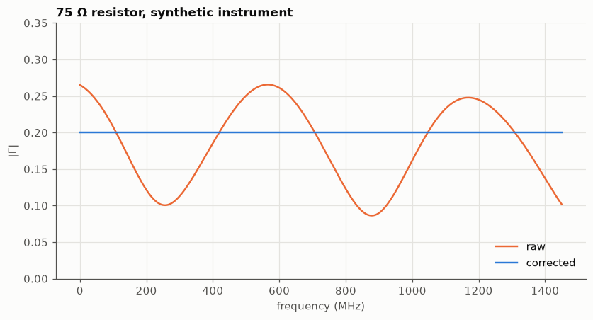
The ripple is gone and the resistor is 75 Ω at every frequency. On synthetic data the result is exact, because the instrument obeys the model perfectly and the standards are perfect. Real data will not be that kind.

The loop above is written to be read. The course package has the same solver without the loop, vnacourse.calibration.solve_error_terms, which solves all frequencies in one call. They give the same answer:

from vnacourse import calibration

package_terms = calibration.solve_error_terms(measured_sol, ideal_sol)
assert all(np.allclose(a, b) for a, b in zip(found_terms, package_terms, strict=True))
assert np.allclose(calibration.correct(gamma_raw, package_terms), gamma_corrected)
print("Same result as vnacourse.calibration")

Same result as vnacourse.calibration

4. Calibrate real measurements

The repository includes the raw readings of a short, an open and a load taken with a NanoVNA-F V2, ten repetitions each (see data/README.md). Averaging the repetitions reduces the random error before we solve for the systematic one.

For now we assume that the three standards are ideal. Section 6 comes back to that assumption.

f_real, short_reps = load_repetitions("standards", "short")
_, open_reps = load_repetitions("standards", "open")
_, load_reps = load_repetitions("standards", "load")
f_real_mhz = f_real / 1e6

ideal = [-1.0, 1.0, 0.0]  # short, open, load
measured = [reps.mean(axis=0) for reps in (short_reps, open_reps, load_reps)]
terms = calibration.solve_error_terms(measured, ideal)

fig, ax = plt.subplots()
ax.semilogy(f_real_mhz, np.abs(terms.directivity), label="directivity $|e_{00}|$")
ax.semilogy(f_real_mhz, np.abs(terms.source_match), label="source match $|e_{11}|$")
ax.semilogy(f_real_mhz, np.abs(terms.tracking), label="tracking $|e_{10}e_{01}|$")
ax.set(xlabel="frequency (MHz)", ylabel="magnitude (log scale)")
ax.set_title("Error terms of the NanoVNA-F V2, from the recorded standards")
ax.legend(loc="upper center", bbox_to_anchor=(0.5, -0.18), ncol=3)

above = f_real > 150e6
print(
    f"Tracking magnitude: up to {np.abs(terms.tracking).max():.2f} below 150 MHz, "
    f"{np.abs(terms.tracking[above]).min():.3f} to {np.abs(terms.tracking[above]).max():.3f} above"
)
print(
    f"Largest source match: {np.abs(terms.source_match).max():.3f} "
    f"at {f_real_mhz[np.abs(terms.source_match).argmax()]:.0f} MHz"
)

Tracking magnitude: up to 1.88 below 150 MHz, 0.994 to 1.015 above
Largest source match: 0.123 at 71 MHz

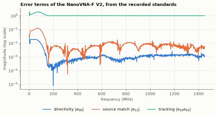
This is the instrument’s own fingerprint. Below about 150 MHz the tracking term is far from 1, which is what made the open and the short read above 1 in notebook 02. Above 150 MHz the tracking stays within a few percent of 1 and the other two terms are small: there the raw reading is already close, and calibration is a fine adjustment.

4.1 Correct two resistors

The same instrument measured a 33 Ω and a 75 Ω resistor, three repetitions each. Their true reflection coefficients are \((33-50)/(33+50) = -0.20\) and \((75-50)/(75+50) = +0.20\).

duts = {}
for label, folder in (("33 Ω", "load_33ohm"), ("75 Ω", "load_75ohm")):
    _, reps = load_repetitions("dut", folder)
    raw = reps.mean(axis=0)
    duts[label] = {"raw": raw, "corrected": calibration.correct(raw, terms)}

low = f_real < 10e6
for label, dut in duts.items():
    z_raw = gamma_to_z(dut["raw"][low]).real
    z_corrected = gamma_to_z(dut["corrected"][low]).real
    print(
        f"{label} resistor below 10 MHz:  raw {z_raw.min():6.1f} to {z_raw.max():6.1f} Ω   "
        f"corrected {z_corrected.min():5.1f} to {z_corrected.max():5.1f} Ω"
    )

33 Ω resistor below 10 MHz:  raw   23.0 to   50.0 Ω   corrected  31.8 to  32.8 Ω
75 Ω resistor below 10 MHz:  raw   38.4 to  101.4 Ω   corrected  73.3 to  75.6 Ω

At low frequency the raw readings are useless and the corrected ones land within a couple of ohms of the nominal values. The calibration works.

Now look at the whole band.

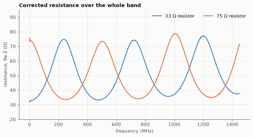
Predict before you run. A resistor has the same resistance at every frequency. What should the corrected \(\operatorname{Re} Z\) look like from 50 kHz to 1.45 GHz?

fig, ax = plt.subplots()
for label, dut in duts.items():
    ax.plot(f_real_mhz, gamma_to_z(dut["corrected"]).real, label=f"{label} resistor")
ax.set(xlabel="frequency (MHz)", ylabel="resistance, Re Z (Ω)", ylim=(20, 95))
ax.set_title("Corrected resistance over the whole band")
ax.legend(loc="upper right", ncol=2);

4.2 The reference plane

Both resistors swing between roughly 33 Ω and 75 Ω, in opposite directions. Is the calibration wrong? Look at the same corrected data on the Smith chart, and at its magnitude.

fig, (ax_smith, ax_mag) = plt.subplots(1, 2, figsize=(10, 4.6))
plotting.gamma_plane(ax_smith, title="Corrected Γ on the Smith chart")
for label, dut in duts.items():
    gamma = dut["corrected"]
    ax_smith.plot(gamma.real, gamma.imag, label=f"{label} resistor")
    ax_mag.plot(f_real_mhz, np.abs(gamma), label=f"{label} resistor")
ax_smith.legend(loc="upper left", bbox_to_anchor=(0.0, 0.0))
ax_mag.set(xlabel="frequency (MHz)", ylabel="$|\\Gamma|$", ylim=(0, 0.4))
ax_mag.set_title("Corrected |Γ|")
ax_mag.legend(loc="lower left");

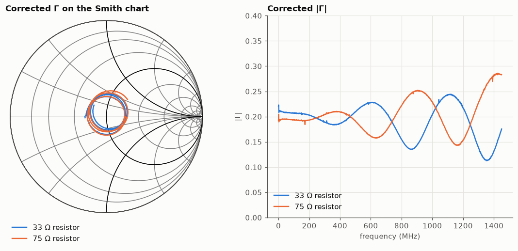
The magnitude stays around 0.2, as it should, with a ripple that grows with frequency. What changes most is the phase: each trace goes around the centre of the chart several times. A reflection coefficient of roughly constant magnitude whose phase falls steadily with frequency is what you see when the device sits at the end of a length of transmission line. A wave that travels a line of one-way delay \(\tau\), reflects, and comes back, arrives with an extra phase \(-2\pi f \cdot 2\tau\):

\[\Gamma_\text{seen} = \Gamma_\text{device}\; e^{-j 4\pi f \tau}\]

Calibration moves the measurement to the reference plane: the exact point where the standards were connected. Everything beyond that point (an adapter, a short cable, the leads of the component) is, for the instrument, part of the device. The data is consistent with a short line between the calibration plane and each resistor.

We can estimate its delay from the slope of the phase, and then remove it.

c0 = 299_792_458.0

fig, ax = plt.subplots()
for label, dut in duts.items():
    gamma = dut["corrected"]
    slope = np.polyfit(f_real, np.unwrap(np.angle(gamma)), 1)[0]  # rad per Hz
    tau = -slope / (4 * np.pi)
    dut["deembedded"] = gamma * np.exp(1j * 4 * np.pi * f_real * tau)

    z = gamma_to_z(dut["deembedded"]).real
    ax.plot(f_real_mhz, z, label=f"{label} resistor")
    print(
        f"{label}: one-way delay {tau * 1e12:.0f} ps, about {tau * c0 * 0.7 * 100:.0f} cm of line "
        f"at 0.7 c;  Re Z after removing it: mean {z.mean():.1f} Ω, "
        f"{z.min():.1f} to {z.max():.1f} Ω"
    )
ax.set(xlabel="frequency (MHz)", ylabel="resistance, Re Z (Ω)", ylim=(0, 100))
ax.set_title("Resistance after moving the reference plane to the resistor")
ax.legend(loc="center right");

33 Ω: one-way delay 1048 ps, about 22 cm of line at 0.7 c;  Re Z after removing it: mean 34.2 Ω, 30.4 to 39.9 Ω
75 Ω: one-way delay 1008 ps, about 21 cm of line at 0.7 c;  Re Z after removing it: mean 75.2 Ω, 66.6 to 89.5 Ω

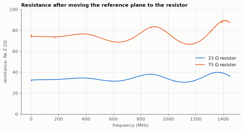
With about 1 ns of line removed, the swing between 33 Ω and 75 Ω is gone: on average the two resistors read within about an ohm of their nominal values. What remains is a slow variation of a few ohms at low frequency that grows to roughly ±10 Ω for the 75 Ω resistor at the top of the band. That is the part a pure delay cannot describe: a line or connector that is not exactly 50 Ω (the ripple in \(|\Gamma|\) above), some loss, and the parasitic inductance and capacitance of a real resistor.

Two lessons:

• A calibration is valid at one plane. Calibrate where the device will be connected, with the same cables and adapters.

• Moving the reference plane afterwards by a delay is a common tool (instruments call it port extension or electrical delay). It is a model, and only as good as the “ideal lossless 50 Ω line” assumption behind it.

4.3 Is the calibration any good?

Correcting the same three measurements you calibrated with proves nothing: the system has three equations and three unknowns, so they come back as exactly −1, +1 and 0 by construction. A fair test uses measurements the calibration has not seen.

We have ten repetitions of each standard. Calibrate with the first five and correct the last five.

train = [reps[:5].mean(axis=0) for reps in (short_reps, open_reps, load_reps)]
test = [reps[5:].mean(axis=0) for reps in (short_reps, open_reps, load_reps)]
terms_train = calibration.solve_error_terms(train, ideal)

fig, ax = plt.subplots()
for name, raw, target in zip(("short", "open", "load"), test, ideal, strict=True):
    residual = np.abs(calibration.correct(raw, terms_train) - target)
    ax.semilogy(f_real_mhz, residual, label=name, linewidth=1.0)
    print(
        f"{name:<5} residual |Γ − ideal|: median {np.median(residual):.4f}, "
        f"worst {residual.max():.3f} "
        f"at {f_real_mhz[residual.argmax()]:.0f} MHz"
    )
ax.set(xlabel="frequency (MHz)", ylabel="$|\\Gamma_{corrected} - \\Gamma_{ideal}|$ (log scale)")
ax.set_title("Residual error on repetitions not used for calibration")
ax.legend(loc="upper center", bbox_to_anchor=(0.5, -0.18), ncol=3)

raw_error = np.abs(test[1] - 1)
print(
    f"\nFor comparison, the raw open is off by {np.median(raw_error):.4f} (median), "
    f"{raw_error.max():.2f} (worst)"
)

short residual |Γ − ideal|: median 0.0015, worst 0.045 at 1 MHz
open  residual |Γ − ideal|: median 0.0016, worst 0.040 at 1311 MHz
load  residual |Γ − ideal|: median 0.0003, worst 0.003 at 0 MHz

For comparison, the raw open is off by 0.0081 (median), 1.93 (worst)

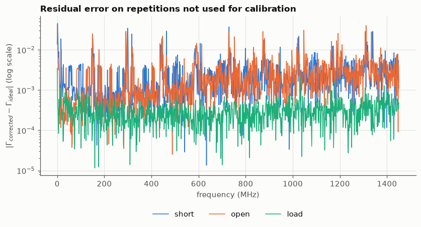
The residual is typically a few thousandths for the short and the open and a few ten-thousandths for the load, with isolated points that are much worse. This residual is not systematic error any more: it is the repeatability of the measurement (noise, and the connection changing slightly between repetitions). Calibration cannot go below it. Notebook 05 looks at repeatability properly.

Note what this test does not check. The same three physical standards are on both sides, so if the “open” is not really \(\Gamma = +1\), this test will not notice. That is section 6.

5. The same calibration with scikit-rf

You will not write this solver every time. scikit-rf implements one-port calibration as skrf.calibration.OnePort. It works with Network objects rather than bare arrays, so we wrap our data first.

frequency = rf.Frequency.from_f(f_real, unit="Hz")


def as_network(gamma, name):
    return rf.Network(
        frequency=frequency,
        s=np.asarray(gamma, dtype=complex) * np.ones(len(f_real)),
        z0=50,
        name=name,
    )


names = ("short", "open", "load")
cal = rf.calibration.OnePort(
    measured=[as_network(m, name) for m, name in zip(measured, names, strict=True)],
    ideals=[as_network(g, name) for g, name in zip(ideal, names, strict=True)],
)
cal.run()

for ours, key in zip(terms, ("directivity", "source match", "reflection tracking"), strict=True):
    print(
        f"{key:<20} largest difference from our solver: {np.abs(cal.coefs[key] - ours).max():.1e}"
    )

corrected_skrf = cal.apply_cal(as_network(duts["75 Ω"]["raw"], "75 ohm")).s[:, 0, 0]
assert np.allclose(corrected_skrf, duts["75 Ω"]["corrected"])
print("The corrected 75 Ω resistor is the same with both")

directivity          largest difference from our solver: 3.5e-16
source match         largest difference from our solver: 6.3e-16
reflection tracking  largest difference from our solver: 2.0e-15
The corrected 75 Ω resistor is the same with both

Same error terms, same corrected result. The library is doing what you did by hand, which means you now know what it is doing. From here on, use whichever is more convenient.

A note on names. The research repository these measurements come from, nanovna-calibration, solves the same system but stores its third unknown as er, with the model written as \(\Gamma_m = (e_d + e_r\Gamma)/(1 - e_s\Gamma)\). Compare with section 1: that er is \(-\Delta_e = e_{10}e_{01} - e_{00}e_{11}\), which is close to the reflection tracking, but not identical to it. The corrected \(\Gamma\) is the same either way. Exercise 3 asks you to check.

6. What if the standards are not ideal?

A calibration tells the instrument “this is \(\Gamma = +1\)”. The instrument believes you. If the open you connected is not really \(+1\), every later measurement inherits that mistake.

Real standards are not ideal. An open has a little capacitance to ground at its end; a short has a little inductance; a load is not exactly 50 Ω. We can try it on the synthetic instrument, where we control the truth: calibrate with slightly imperfect standards, once pretending they are ideal and once telling the solver what they really are.

omega = 2 * np.pi * f_hz
real_short = z_to_gamma(1j * omega * 0.3e-9)  # 0.3 nH in series
real_open = z_to_gamma(1 / (1j * omega * 0.1e-12))  # 0.1 pF to ground
real_load = z_to_gamma(51.5) * ones  # 51.5 Ω instead of 50 Ω
real_sol = [real_short, real_open, real_load]

measured_real_sol = [apply_error_model(gamma, true_terms) for gamma in real_sol]
terms_assumed_ideal = solve_error_terms(measured_real_sol, ideal_sol)
terms_defined = solve_error_terms(measured_real_sol, real_sol)

wrong = gamma_to_z(correct(gamma_raw, terms_assumed_ideal))
right = gamma_to_z(correct(gamma_raw, terms_defined))

fig, (ax_re, ax_im) = plt.subplots(1, 2, figsize=(10, 3.8))
for ax, part, name in (
    (ax_re, np.real, "resistance, Re Z (Ω)"),
    (ax_im, np.imag, "reactance, Im Z (Ω)"),
):
    ax.plot(f_mhz, part(wrong), color=plotting.SERIES[1], label="standards assumed ideal")
    ax.plot(f_mhz, part(right), color=plotting.SERIES[0], label="standards described as they are")
    ax.set(xlabel="frequency (MHz)", ylabel=name)
ax_re.set_ylim(70, 76)
ax_im.set_ylim(-1, 4)
ax_re.set_title("75 Ω resistor after calibrating with imperfect standards")
ax_im.legend(loc="upper left")

print(
    f"Assumed ideal: Re Z from {wrong.real.min():.1f} to {wrong.real.max():.1f} Ω, "
    f"Im Z from {wrong.imag.min():.1f} to {wrong.imag.max():.1f} Ω"
)

Assumed ideal: Re Z from 72.6 to 72.8 Ω, Im Z from 0.0 to 2.8 Ω

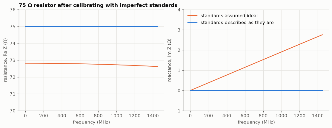
With the standards described correctly the result is exact again. With the “ideal” assumption the resistance is more than 2 Ω low at every frequency (the load was 51.5 Ω, and we called it 50 Ω), and the resistor gains a reactance it does not have, which grows with frequency because 0.1 pF and 0.3 nH matter more and more.

This is why a calibration kit comes with a definition: numbers that describe how each standard really behaves (delay, fringing capacitance, inductance). The solver you wrote already accepts them: actual can be any known \(\Gamma\), not only −1, +1 and 0. For the real data in section 4 we have no such definition, so we assumed ideal standards, and that assumption sets a limit on the accuracy of everything we corrected.

Check your understanding

1. With ideal standards the system has a simple closed form. What is \(e_{00}\)?

Answer

Put \(\Gamma = 0\) in the model: \(\Gamma_m = e_{00}\). The directivity is simply the raw reading of the load. The short and the open then give two equations for the other two terms.

2. You calibrate, then add a 10 cm cable between the port and your device. Which of your results are still right: \(|\Gamma|\), the phase of \(\Gamma\), the impedance?

Answer

If the cable were a perfect, lossless 50 Ω line, \(|\Gamma|\) would still be right and the phase would not, so the impedance would be wrong (section 4.2). A real cable also has loss and its own mismatch, so even \(|\Gamma|\) degrades. The correct procedure is to calibrate at the end of the cable.

3. Why is “correct the standards and check that you get −1, +1 and 0” not a valid test of a calibration?

Answer

Three equations, three unknowns: the solution reproduces the three calibration measurements exactly, whatever they were. You would get −1, +1 and 0 even if you had connected the wrong parts. A test needs independent data: other repetitions (section 4.3) or, better, a different known device.

4. In section 4.3 the load has a much smaller residual than the short and the open. Suggest a reason.

Answer

Tracking and source-match errors, and any change in them between repetitions, are multiplied by \(\Gamma\). For the load \(\Gamma \approx 0\), so they hardly show; for the short and the open \(|\Gamma| = 1\), so they show in full.

Exercises

Worked solutions are in exercises/solutions/03_solutions.ipynb.

1. Closed form. For ideal standards, derive \(e_{11}\) and \(e_{10}e_{01}\) by hand from the short and open equations, implement them without np.linalg.solve, and check against solve_error_terms on the real data.

2. Fewer repetitions. Repeat section 4.3 calibrating with a single repetition instead of five. How does the median residual change? What does that say about the value of averaging?

3. Two parametrisations. Compute er = tracking - directivity * source_match from the real error terms. Plot \(|e_r|\) and \(|e_{10}e_{01}|\) together. Where do they differ most, and why there? Then verify that \((\Gamma_m - e_d)/(e_r + e_s\Gamma_m)\) gives the same corrected \(\Gamma\) as correct.

4. A fourth standard. Add the 75 Ω resistor as a fourth known device on the synthetic instrument. The system now has four equations and three unknowns. Solve it with np.linalg.lstsq. Add a little random noise to the four “measurements” and compare the error of the three-standard and four-standard solutions.

5. How much does the open matter? In section 6, change the fringing capacitance of the open from 0.1 pF to 0.05 pF and to 0.2 pF. At 1.45 GHz, how many ohms of error in the 75 Ω resistor does each value cause?

# Your work here

Summary

• Multiplying the error model by its denominator makes it linear in \(e_{00}\), \(e_{11}\) and \(\Delta_e = e_{00}e_{11} - e_{10}e_{01}\). Three known standards give a 3×3 system per frequency.

• The correction is \(\Gamma = \dfrac{\Gamma_m - e_{00}}{e_{10}e_{01} + e_{11}(\Gamma_m - e_{00})}\).

• On synthetic data the calibration is exact. On real data it is limited by repeatability and by how well you know your standards.

• A calibration is valid at the plane where the standards were connected. Anything added after that is measured as part of the device.

• skrf.calibration.OnePort does the same computation.

Next: 05 · Validation and measurement quality asks how much to trust these results. (Notebook 04, on acquiring your own measurements with a NanoVNA, is optional and not yet available.)