01 · Reflection coefficient and the Smith chart

A VNA gives you a reflection coefficient \(\Gamma\) at each frequency. What you usually want to know is an impedance: is this electrode capacitive? where does this coil resonate? is this antenna matched? The two are linked by a simple formula, and the Smith chart is the picture of that formula. In this notebook you build the chart yourself and learn to read circuits from the shape of a trace.

Learning objectives

After this notebook you will be able to:

• convert between impedance \(Z\) and reflection coefficient \(\Gamma\) in both directions;

• explain what the circles and arcs of a Smith chart are, and locate any impedance on it;

• recognise resistive, inductive and capacitive behaviour, and resonance, from a trace;

• identify a simple circuit from its trace across frequency.

You need: notebook 00, and the impedance of R, L and C in sinusoidal steady state. No hardware.

import sys

if "google.colab" in sys.modules:
    %pip install -q git+https://github.com/telmomm/nanovna-measurement-course

import matplotlib.pyplot as plt
import numpy as np

from vnacourse import plotting
from vnacourse.puzzles import mystery_trace

plotting.use_course_style()

1. From impedance to reflection, and back

For a load \(Z\) on a port of reference impedance \(Z_0 = 50\ \Omega\):

\[\Gamma = \frac{Z - Z_0}{Z + Z_0} \qquad\Longleftrightarrow\qquad Z = Z_0\,\frac{1 + \Gamma}{1 - \Gamma}\]

Each impedance corresponds to exactly one point of the complex \(\Gamma\) plane, and the other way round. Write both functions:

Z0 = 50.0


def z_to_gamma(z):
    """Reflection coefficient of an impedance z on a 50 Ω port."""
    z = np.asarray(z, dtype=complex)
    return (z - Z0) / (z + Z0)


def gamma_to_z(gamma):
    """Impedance that produces the reflection coefficient gamma on a 50 Ω port."""
    gamma = np.asarray(gamma, dtype=complex)
    return Z0 * (1 + gamma) / (1 - gamma)


print(z_to_gamma(75))
print(gamma_to_z(0.2))

(0.2+0j)
(75+0j)

Predict before you run. Where on the \(\Gamma\) plane do these land: a short (0 Ω), a matched load (50 Ω), a 150 Ω resistor, a pure inductive reactance \(+j50\ \Omega\), a pure capacitive reactance \(-j50\ \Omega\)? Sketch it on paper first. The open circuit (\(Z \to \infty\)) is at \(\Gamma = +1\).

landmarks = {
    "short": 0,
    "16.7 Ω": 50 / 3,
    "50 Ω": 50,
    "150 Ω": 150,
    "+j50 Ω": 50j,
    "−j50 Ω": -50j,
    "50 + j50 Ω": 50 + 50j,
}

fig, ax = plt.subplots(figsize=(5.4, 5.4))
plotting.gamma_plane(ax, radius=1.25, title="Some impedances on the Γ plane")
print(f"{'impedance':>12}  {'Γ':>16}  {'|Γ|':>5}  {'angle':>7}")
for name, z in landmarks.items():
    gamma = z_to_gamma(z)
    ax.plot(gamma.real, gamma.imag, "o", color=plotting.SERIES[0])
    ax.annotate(
        name, (gamma.real, gamma.imag), xytext=(0, 9), textcoords="offset points", ha="center"
    )
    print(f"{name:>12}  {gamma:16.2f}  {abs(gamma):5.2f}  {np.degrees(np.angle(gamma)):6.0f}°")
ax.plot(1, 0, "o", color=plotting.SERIES[0])
ax.annotate("open", (1, 0), xytext=(0, 9), textcoords="offset points", ha="center");

   impedance                 Γ    |Γ|    angle
       short       -1.00+0.00j   1.00     180°
      16.7 Ω       -0.50+0.00j   0.50     180°
        50 Ω        0.00+0.00j   0.00       0°
       150 Ω        0.50+0.00j   0.50       0°
      +j50 Ω        0.00+1.00j   1.00      90°
      −j50 Ω        0.00-1.00j   1.00     -90°
  50 + j50 Ω        0.20+0.40j   0.45      63°

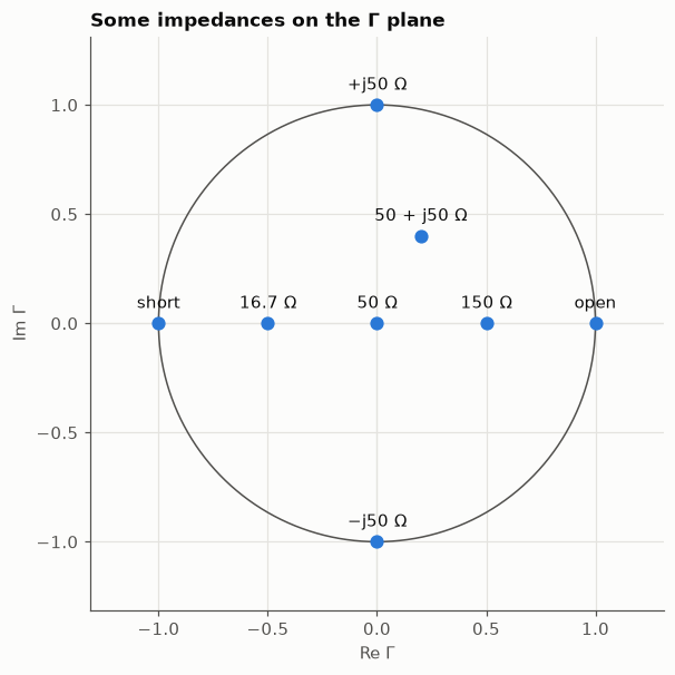
Four things to notice:

• Resistors lie on the horizontal axis: below 50 Ω to the left, above 50 Ω to the right, 50 Ω at the centre.

• 16.7 Ω and 150 Ω are \(Z_0/3\) and \(3Z_0\): they land at −0.5 and +0.5, mirror images.

• Pure reactances lie on the circle \(|\Gamma| = 1\): they reflect everything, because a reactance dissipates no power.

• Inductive impedances (positive reactance) are in the upper half, capacitive ones in the lower half.

The whole right half of the impedance plane (every impedance with \(R \ge 0\)) fits inside the unit circle. That is the point of working with \(\Gamma\): every passive load, from short to open, lives in a finite disc.

2. Build the Smith chart

The Smith chart is the \(\Gamma\) plane with a grid drawn on it. The grid lines are the images of the simplest lines of the impedance plane:

• all impedances with the same resistance \(R\) and any reactance;

• all impedances with the same reactance \(X\) and any resistance.

Predict before you run. A vertical line in the impedance plane (\(R\) fixed, \(X\) from \(-\infty\) to \(+\infty\)) becomes what shape on the \(\Gamma\) plane?

fig, (ax_r, ax_x) = plt.subplots(1, 2, figsize=(10, 5.2))

reactance = np.concatenate([-np.logspace(4, -2, 400), [0], np.logspace(-2, 4, 400)])
plotting.gamma_plane(ax_r, radius=1.15, title="Constant resistance")
for resistance in (0, 16.7, 50, 150):
    gamma = z_to_gamma(resistance + 1j * reactance)
    ax_r.plot(gamma.real, gamma.imag, label=f"R = {resistance:g} Ω")
ax_r.legend(loc="upper left", bbox_to_anchor=(0.0, -0.12), ncol=2)

resistance = np.logspace(-2, 4, 400)
plotting.gamma_plane(ax_x, radius=1.15, title="Constant reactance")
for x in (50, 150, -50, -150):
    gamma = z_to_gamma(resistance + 1j * x)
    ax_x.plot(gamma.real, gamma.imag, label=f"X = {x:+g} Ω")
ax_x.legend(loc="upper left", bbox_to_anchor=(0.0, -0.12), ncol=2);

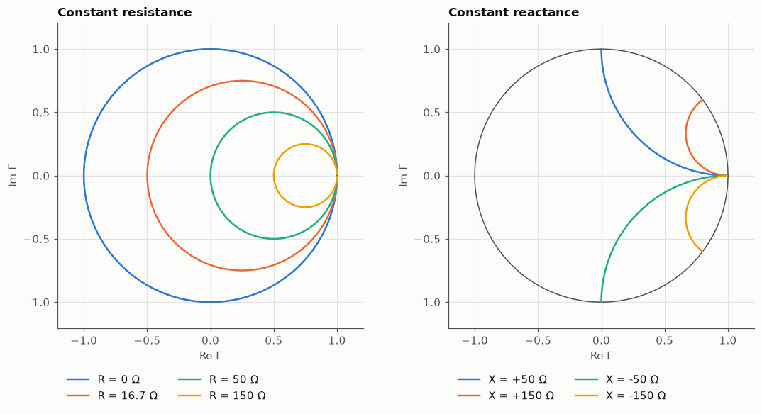
• Lines of constant resistance become circles, all touching the point \(\Gamma = +1\) (the open circuit). \(R = 0\) is the outer circle; \(R = 50\ \Omega\) passes through the centre; larger \(R\) gives smaller circles squeezed towards the right.

• Lines of constant reactance become arcs that also leave from \(\Gamma = +1\): upwards for inductive, downwards for capacitive.

Draw many of both and you have the Smith chart. From now on the course helper draws it for you: plotting.gamma_plane(ax). To read a point, find which resistance circle and which reactance arc pass through it.

Charts are usually labelled with the normalised impedance \(z = Z/Z_0\), so the same chart serves any \(Z_0\): the circle “1” is \(R = Z_0\).

3. Traces: what a circuit looks like across frequency

A resistor is one point. As soon as there is an inductor or a capacitor, the impedance changes with frequency and the point moves, drawing a trace. The shape of the trace tells you the circuit.

We sweep from 10 MHz to 1.45 GHz. The helper below draws traces and marks where each one starts (lowest frequency) with a dot.

f_hz = np.linspace(10e6, 1.45e9, 600)
omega = 2 * np.pi * f_hz


def show(traces, title):
    """Draw traces {label: impedance array} on a Smith chart; a dot marks the lowest frequency."""
    fig, ax = plt.subplots(figsize=(5.4, 5.4))
    plotting.gamma_plane(ax, title=title)
    for label, z in traces.items():
        gamma = z_to_gamma(z)
        (line,) = ax.plot(gamma.real, gamma.imag, label=label)
        ax.plot(gamma[0].real, gamma[0].imag, "o", color=line.get_color())
    ax.legend(loc="upper left", bbox_to_anchor=(0.0, 0.0))
    return ax

3.1 Series circuits

A 25 Ω resistor in series with an inductor, and the same resistor in series with a capacitor:

\[Z_{RL} = R + j\omega L \qquad\qquad Z_{RC} = R + \frac{1}{j\omega C}\]

Predict before you run. The resistance is 25 Ω at every frequency. Along which grid line will both traces move? In which half of the chart is each one, and where does each one start?

R = 25.0
z_series_rl = R + 1j * omega * 10e-9  # 10 nH
z_series_rc = R + 1 / (1j * omega * 5e-12)  # 5 pF

show(
    {"25 Ω + 10 nH in series": z_series_rl, "25 Ω + 5 pF in series": z_series_rc},
    "Series RL and RC",
);

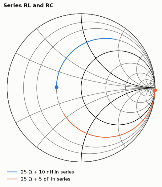
Both traces stay on the 25 Ω resistance circle, because the resistance never changes.

• The RL trace starts at the resistor (at low frequency the inductor is a short) and climbs into the upper, inductive half as \(\omega L\) grows.

• The RC trace starts near the open circuit (at low frequency the capacitor blocks) and comes down the lower, capacitive half towards the resistor as \(1/\omega C\) shrinks.

Both move clockwise as frequency increases. That is true of every trace of a passive circuit made of R, L and C, and it is a quick sanity check on any measurement.

3.2 Parallel circuits

Now a 100 Ω resistor in parallel with the same kind of element. In parallel, admittances add:

\[\frac{1}{Z} = \frac{1}{R} + \frac{1}{j\omega L} \qquad\qquad \frac{1}{Z} = \frac{1}{R} + j\omega C\]

Predict before you run. At low frequency, what does an inductor in parallel with a resistor look like? And a capacitor in parallel with a resistor at high frequency?

R = 100.0
z_parallel_rl = 1 / (1 / R + 1 / (1j * omega * 20e-9))  # 20 nH
z_parallel_rc = 1 / (1 / R + 1j * omega * 3e-12)  # 3 pF

show({"100 Ω ∥ 20 nH": z_parallel_rl, "100 Ω ∥ 3 pF": z_parallel_rc}, "Parallel RL and RC");

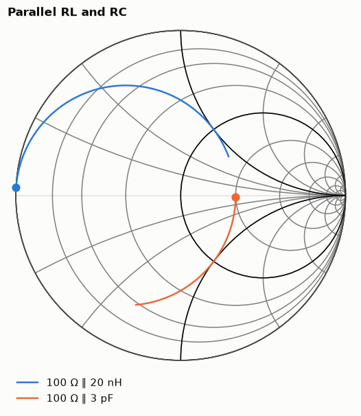
• The parallel RL starts near the short (the inductor shorts the resistor at low frequency) and travels through the inductive half towards the 100 Ω point.

• The parallel RC starts at the 100 Ω point and heads through the capacitive half towards the short (the capacitor shorts the resistor at high frequency).

These traces do not follow a constant-resistance circle. They follow a circle that touches the short instead of the open: a circle of constant conductance, \(G = 1/R\). It is the mirror image of a resistance circle. Series elements move you along resistance circles; parallel elements move you along conductance circles.

3.3 Resonance

Put an inductor and a capacitor in series with a resistor:

\[Z = R + j\left(\omega L - \frac{1}{\omega C}\right)\]

The two reactances have opposite signs and cancel at the resonant frequency \(f_0 = \dfrac{1}{2\pi\sqrt{LC}}\).

Predict before you run. Where on the chart is the trace at \(f_0\)? In which half is it below \(f_0\), and above?

R, L, C = 25.0, 20e-9, 5e-12
z_series_rlc = R + 1j * omega * L + 1 / (1j * omega * C)
f0 = 1 / (2 * np.pi * np.sqrt(L * C))

ax = show({"25 Ω + 20 nH + 5 pF in series": z_series_rlc}, "Series RLC")
gamma_f0 = z_to_gamma(R)
ax.plot(gamma_f0.real, gamma_f0.imag, "s", color=plotting.INK)
ax.annotate("$f_0$", (gamma_f0.real, gamma_f0.imag), xytext=(-14, 8), textcoords="offset points")

fig, ax = plt.subplots()
ax.plot(f_hz / 1e6, np.abs(z_to_gamma(z_series_rlc)))
ax.axvline(f0 / 1e6, color=plotting.INK_SECONDARY, linewidth=0.8, linestyle="--")
ax.set(xlabel="frequency (MHz)", ylabel="$|\\Gamma|$", ylim=(0, 1.05))
ax.set_title("Series RLC: magnitude of the reflection")

print(f"Resonant frequency: {f0 / 1e6:.0f} MHz")
print(f"|Γ| at resonance: {abs(gamma_f0):.3f}")

Resonant frequency: 503 MHz
|Γ| at resonance: 0.333

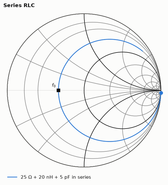
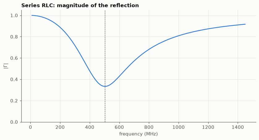
The trace runs along the 25 Ω circle: capacitive (lower half) below resonance, inductive (upper half) above, and it crosses the horizontal axis at \(f_0\), where the impedance is the bare resistance. On the magnitude plot, resonance is the dip: the reflection is smallest where the reactance vanishes.

Reading a resonance off a chart: the crossing of the real axis gives you \(f_0\) and the resistance at once. The magnitude plot gives you only \(f_0\).

3.4 A resistor behind a cable

One more shape, from notebook 00: a 75 Ω resistor at the end of 20 cm of cable. The cable does not change \(|\Gamma|\), it only rotates the phase.

tau = 0.20 / (0.7 * 299_792_458.0)
gamma_cable = z_to_gamma(75) * np.exp(-4j * np.pi * f_hz * tau)

ax = show(
    {"75 Ω behind 20 cm of cable": gamma_to_z(gamma_cable)},
    "A delay draws a circle around the centre",
)

z_seen = gamma_to_z(gamma_cable)
print(f"Resistance seen at the port: from {z_seen.real.min():.1f} Ω to {z_seen.real.max():.1f} Ω")

Resistance seen at the port: from 33.3 Ω to 75.0 Ω

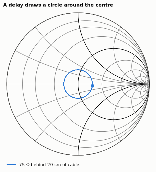
A circle centred on the centre of the chart means constant \(|\Gamma|\) and rotating phase: the signature of a length of line in front of the device. Through the cable, the 75 Ω resistor looks like anything between 33 Ω and 75 Ω, with reactance, depending on frequency. You will meet exactly this in real data in notebook 03.

Shape of the trace	Circuit
a point on the horizontal axis	resistor
arc along a resistance circle, upper half	R in series with L
arc along a resistance circle, lower half	R in series with C
arc along a conductance circle (touching the short)	R in parallel with L or C
crosses the horizontal axis	resonance
circle around the centre	a length of line in front of the device

4. Guess the circuit

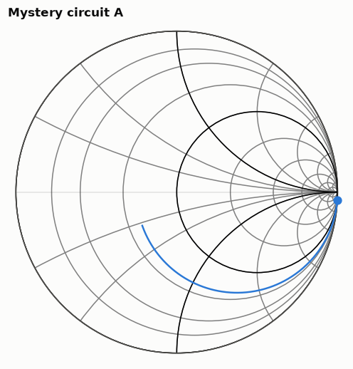
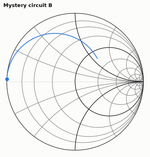
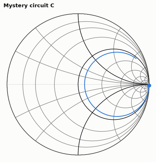
Three mystery circuits, each made of one resistor and one or two reactive elements. mystery_trace("A", f_hz) returns the reflection coefficient of circuit A. Use what you learned:

1. Where does the trace start and where does it end? What is the circuit at very low and very high frequency?

2. Does it follow a resistance circle or a conductance circle?

3. Does it cross the horizontal axis?

Then convert to impedance with gamma_to_z and read the values. Decide on a topology before you compute anything.

for name in ("A", "B", "C"):
    gamma = mystery_trace(name, f_hz)
    fig, ax = plt.subplots(figsize=(4.6, 4.6))
    plotting.gamma_plane(ax, title=f"Mystery circuit {name}")
    ax.plot(gamma.real, gamma.imag, color=plotting.SERIES[0])
    ax.plot(gamma[0].real, gamma[0].imag, "o", color=plotting.SERIES[0])

# Work out the circuits here. For example, the impedance of A at the highest frequency:
z_a = gamma_to_z(mystery_trace("A", f_hz))
print(f"Z of A at {f_hz[-1] / 1e6:.0f} MHz: {z_a[-1]:.1f} Ω")

Z of A at 1450 MHz: 30.0-13.7j Ω

Check your understanding

1. Where is \(Z = 50 - j50\ \Omega\) on the chart? Give \(|\Gamma|\) and the half of the chart.

Answer

\(\Gamma = \dfrac{-j50}{100 - j50} = 0.2 - 0.4j\), so \(|\Gamma| = 0.45\), in the lower (capacitive) half, on the \(R = 50\ \Omega\) circle that passes through the centre.

2. A trace starts at the short, runs through the upper half of the chart and ends on the horizontal axis at the 100 Ω point. What is the circuit?

Answer

A 100 Ω resistor in parallel with an inductor. At low frequency the inductor shorts the resistor (the trace starts at the short); at high frequency the inductor is an open circuit and only the resistor is left. The upper half confirms an inductive element, and the path is a conductance circle, as for every parallel element.

3. Why do all traces of passive circuits stay inside the unit circle?

Answer

\(|\Gamma| > 1\) would mean more power reflected than received. A passive circuit has \(R \ge 0\), and every impedance with \(R \ge 0\) maps inside or onto the circle \(|\Gamma| = 1\).

4. On the magnitude plot of the series RLC, how would the dip change if the resistor were 50 Ω instead of 25 Ω?

Answer

At resonance \(Z = R = 50\ \Omega\), so \(\Gamma = 0\): the dip would go all the way to zero. The trace would pass through the centre of the chart. That is a matched resonant circuit.

Exercises

Worked solutions are in exercises/solutions/01_solutions.ipynb.

1. There and back. Compute \(\Gamma\) for \(Z = 20 - j30\ \Omega\) by hand, check with z_to_gamma, and convert back. Then find the impedance at \(\Gamma = 0.5\angle 90°\).

2. Admittance. Show numerically that the reflection coefficient of the admittance-mirrored load, \(Z' = Z_0^2 / Z\), is \(-\Gamma\): the same point rotated by 180°. Use it to explain why conductance circles are mirror images of resistance circles.

3. Parallel resonance. Plot the trace of 100 Ω ∥ 5 nH ∥ 20 pF. Where is it at resonance? In which half is it below resonance: the opposite of the series case, or the same?

4. The mystery circuits. For A, B and C give the topology and estimate the component values from the trace.

# Your work here

Summary

• \(\Gamma = (Z - Z_0)/(Z + Z_0)\) maps every passive impedance into the unit disc: short at −1, match at 0, open at +1.

• The Smith chart is that disc with circles of constant resistance and arcs of constant reactance.

• Upper half inductive, lower half capacitive, horizontal axis resistive, rim purely reactive.

• Traces of passive circuits move clockwise with frequency. Series elements follow resistance circles, parallel elements follow conductance circles, and a resonance crosses the horizontal axis.

• A circle around the centre is a delay: a line in front of the device.

Next: in 02 · Systematic errors you find out that the \(\Gamma\) an instrument reports is not the \(\Gamma\) of the device.