Solutions · 02 Systematic errors

Worked solutions to the exercises of notebook 02. Try each exercise yourself first.

import sys

if "google.colab" in sys.modules:
    %pip install -q git+https://github.com/telmomm/nanovna-measurement-course

import matplotlib.pyplot as plt
import numpy as np

from vnacourse import plotting
from vnacourse.data import load_repetitions
from vnacourse.errormodel import ErrorTerms, apply_error_model, synthetic_error_terms
from vnacourse.reflection import z_to_gamma

plotting.use_course_style()

f_hz = np.linspace(50e3, 1.45e9, 401)
f_mhz = f_hz / 1e6
terms = synthetic_error_terms(f_hz)

1. Which term is to blame?

Build four instruments: the full one, and three with one term made perfect. ErrorTerms is a named tuple, so _replace gives a copy with one field changed. The size of the ripple is the difference between the highest and the lowest reading.

zeros = np.zeros(f_hz.shape, dtype=complex)
instruments = {
    "all three terms": terms,
    "no directivity": terms._replace(directivity=zeros),
    "no source match": terms._replace(source_match=zeros),
    "perfect tracking": terms._replace(tracking=zeros + 1),
}

fig, axes = plt.subplots(1, 2, figsize=(10, 4.2), sharex=True)
for ax, (device, gamma) in zip(
    axes, (("75 Ω resistor", z_to_gamma(75)), ("short", -1.0)), strict=True
):
    print(device)
    for name, instrument in instruments.items():
        measured = np.abs(apply_error_model(gamma + zeros, instrument))
        ax.plot(f_mhz, measured, label=name)
        print(f"   {name:<17} ripple {measured.max() - measured.min():.3f}")
    ax.set(xlabel="frequency (MHz)", ylabel="$|\\Gamma_m|$")
    ax.set_title(device)
axes[0].legend(loc="upper center", bbox_to_anchor=(1.1, -0.18), ncol=4);

75 Ω resistor
   all three terms   ripple 0.179
   no directivity    ripple 0.040
   no source match   ripple 0.168
   perfect tracking  ripple 0.154
short
   all three terms   ripple 0.555
   no directivity    ripple 0.447
   no source match   ripple 0.258
   perfect tracking  ripple 0.543

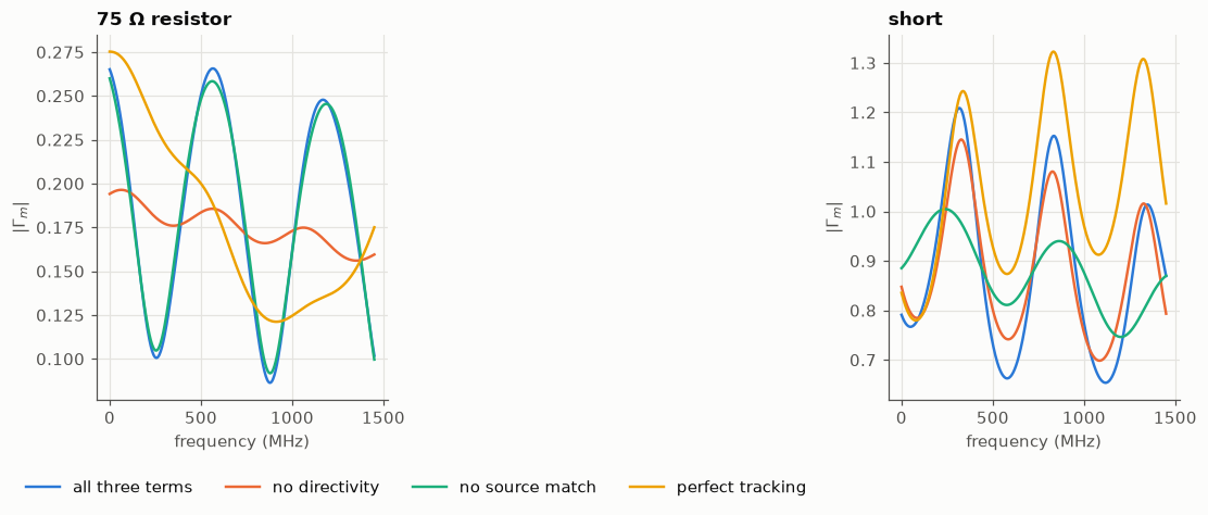
• 75 Ω resistor: removing the directivity makes the ripple collapse from 0.18 to 0.04. Removing the source match changes almost nothing. For a small reflection, directivity is the term that matters: it is a vector of size 0.08 added to a reflection of size 0.2.

• Short: now removing the source match has the biggest effect, halving the ripple. Directivity still contributes, but 0.08 is small next to a reflection of size 1, while the source-match term \(e_{11}\Gamma\) is at its largest.

• Making the tracking perfect changes the shape of the ripple more than its size. The delay in the tracking term is what makes the reflection rotate quickly against the directivity; without it the two vectors still add and cancel, only more slowly with frequency.

The answer to “which error matters most” depends on the device. This is the table of section 2.3 again, seen across frequency.

2. Ripple and length

An instrument whose only flaw is a source match \(0.2\,e^{-j2\pi f\tau}\), measuring a short. We sweep a wider band so that several ripples fit, and find the peaks as the points higher than both neighbours.

f_wide = np.linspace(1e6, 6e9, 6001)

fig, ax = plt.subplots()
for tau in (0.5e-9, 1e-9, 2e-9):
    instrument = ErrorTerms(
        directivity=0, source_match=0.2 * np.exp(-2j * np.pi * f_wide * tau), tracking=1
    )
    measured = np.abs(apply_error_model(-1.0, instrument))
    ax.plot(f_wide / 1e9, measured, label=f"τ = {tau * 1e9:g} ns")

    peaks = np.flatnonzero((measured[1:-1] > measured[:-2]) & (measured[1:-1] > measured[2:])) + 1
    spacing = np.diff(f_wide[peaks]).mean()
    print(
        f"τ = {tau * 1e9:g} ns: peaks {spacing / 1e6:.0f} MHz apart;  1/τ = {1 / tau / 1e6:.0f} MHz"
    )
ax.set(xlabel="frequency (GHz)", ylabel="$|\\Gamma_m|$ of a short")
ax.set_title("Ripple for three delays of the source match")
ax.legend(loc="upper center", bbox_to_anchor=(0.5, -0.18), ncol=3);

τ = 0.5 ns: peaks 2000 MHz apart;  1/τ = 2000 MHz
τ = 1 ns: peaks 1000 MHz apart;  1/τ = 1000 MHz
τ = 2 ns: peaks 500 MHz apart;  1/τ = 500 MHz

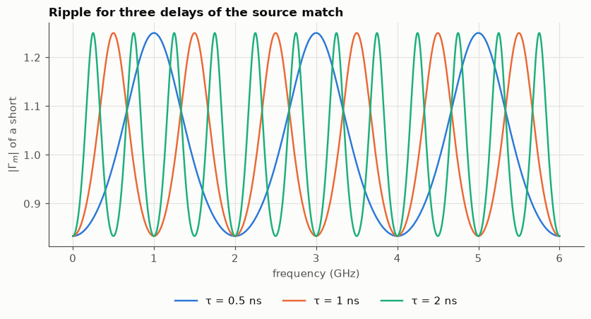
The peaks are \(1/\tau\) apart: the ripple repeats each time the phase of \(e_{11}\) completes a turn. The depth of the ripple is the same in the three cases (it depends on \(|e_{11}|\)), only its spacing changes.

On a real instrument, \(\tau\) is the delay between the DUT and the place where the re-reflection happens. A long cable means a large \(\tau\) and therefore a fine, closely spaced ripple. You can turn this round: measure the spacing of a ripple and you know how far away the mismatch that causes it is. With \(\tau\) as a round-trip delay in a cable at \(0.7c\), a ripple every 100 MHz points to a mismatch about 1 m away.

3. Worst case

The reading is the sum of two vectors of length 0.1 (the device) and 0.03 (the directivity), with unknown relative phase. It is largest when they are aligned and smallest when they are opposed.

gamma_true, directivity = 0.1, 0.03
for label, reading in (
    ("smallest reading", gamma_true - directivity),
    ("true value", gamma_true),
    ("largest reading", gamma_true + directivity),
):
    print(f"{label:<17} |Γ| = {reading:.2f}   return loss = {-20 * np.log10(reading):.1f} dB")

smallest reading  |Γ| = 0.07   return loss = 23.1 dB
true value        |Γ| = 0.10   return loss = 20.0 dB
largest reading   |Γ| = 0.13   return loss = 17.7 dB

A device with 20 dB of return loss may read anything from 17.7 dB to 23.1 dB. The error is not symmetric in decibels, and it grows quickly as the device gets better: for a true return loss of 30 dB (\(|\Gamma| = 0.032\)), a directivity of 0.03 makes the reading meaningless. The directivity of an instrument, after calibration, sets the best match it can certify.

4. Real data

f_real, open_raw = load_repetitions("standards", "open")
_, short_raw = load_repetitions("standards", "short")
f_real_mhz = f_real / 1e6

fig, (ax_phase, ax_reps) = plt.subplots(1, 2, figsize=(10, 4.2))
ax_phase.plot(f_real_mhz, np.degrees(np.angle(open_raw.mean(axis=0))), label="open (ideal: 0°)")
ax_phase.plot(
    f_real_mhz,
    np.degrees(np.angle(-short_raw.mean(axis=0))),
    label="short, minus 180° (ideal: 0°)",
)
ax_phase.set(xlabel="frequency (MHz)", ylabel="phase error (°)")
ax_phase.set_title("Phase of the raw standards")
ax_phase.legend(loc="lower right")

for repetition in open_raw:
    ax_reps.plot(f_real_mhz, np.abs(repetition), color=plotting.SERIES[0], linewidth=0.6)
ax_reps.set(xlabel="frequency (MHz)", ylabel="$|\\Gamma_m|$")
ax_reps.set_title("Raw open: the ten repetitions")

above = f_real > 150e6
phase_open = np.degrees(np.angle(open_raw.mean(axis=0)))
print(
    f"Open phase: {phase_open.min():.0f}° to {phase_open.max():.0f}° over the whole band, "
    f"within ±{np.abs(phase_open[above]).max():.1f}° above 150 MHz"
)

difference = np.abs(np.abs(open_raw) - np.abs(open_raw.mean(axis=0)))
print(
    f"Repetitions differ from their mean by {np.median(difference):.4f} (typical), "
    f"{difference.max():.2f} (worst)"
)

Open phase: -101° to 45° over the whole band, within ±1.1° above 150 MHz
Repetitions differ from their mean by 0.0008 (typical), 0.14 (worst)

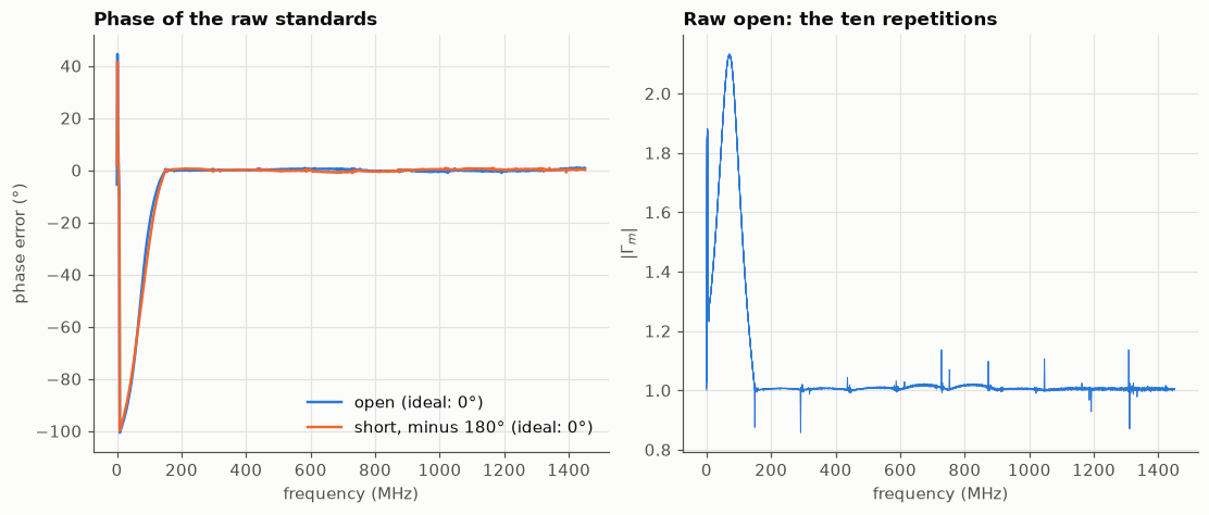
The phase tells the same story as the magnitude. Below about 150 MHz it is off by up to 100°; above, it stays within about 1° of the ideal value. A phase error is the argument of the tracking term (section 2.2).

The ten repetitions lie on top of each other: at this scale you cannot tell them apart, and their typical difference is below 0.001. That is the point of the exercise. The large error is perfectly repeatable, so it is systematic, and repeating the measurement does nothing to reveal it. The few visible spikes are a different matter, studied in notebook 05.