Solutions · 00 What does a VNA measure?

Worked solutions to the exercises of notebook 00. Try each exercise yourself before reading its solution: the attempt is where the learning happens.

import sys

if "google.colab" in sys.modules:
    %pip install -q git+https://github.com/telmomm/nanovna-measurement-course

import matplotlib.pyplot as plt
import numpy as np

from vnacourse import plotting

plotting.use_course_style()

c0 = 299_792_458.0
v = 0.7 * c0
z0 = 50.0


def reflection(z_load):
    return (z_load - z0) / (z_load + z0)

1. How short is short?

A length \(\ell\) is a tenth of a wavelength when \(\lambda = 10\,\ell\), that is at \(f = v / (10\,\ell)\).

for name, length in (("10 cm cable", 0.10), ("1 cm lead", 0.01)):
    f_tenth = v / (10 * length)
    print(f"{name}: a tenth of a wavelength at {f_tenth / 1e6:.0f} MHz")

print(f"\nAt 1 GHz the wavelength in the cable is {v / 1e9 * 100:.0f} cm")
print(f"so a 1 cm lead is 1/{v / 1e9 / 0.01:.0f} of a wavelength")

10 cm cable: a tenth of a wavelength at 210 MHz
1 cm lead: a tenth of a wavelength at 2099 MHz

At 1 GHz the wavelength in the cable is 21 cm
so a 1 cm lead is 1/21 of a wavelength

A 10 cm cable stops being “just a wire” at about 210 MHz, and a 1 cm component lead at about 2.1 GHz. At 1 GHz a 1 cm lead is already a twenty-first of a wavelength: not yet a transmission line, but no longer negligible. At these frequencies the leads, the connector and the way the part is mounted are part of what you measure. This is why RF components are tiny and why the reference plane of notebook 03 matters.

2. Open circuit

An open has \(\Gamma = +1\). Add it to the standing-wave plot.

f = 300e6
beta = 2 * np.pi * f / v
d = np.linspace(0, 1.0, 500)

fig, ax = plt.subplots()
for name, gamma in (("short  (Γ = −1)", -1.0), ("open  (Γ = +1)", 1.0)):
    ax.plot(d, np.abs(1 + gamma * np.exp(-2j * beta * d)), label=name)
ax.set(xlabel="distance from the load (m)", ylabel="voltage amplitude, $|V| / |V^+|$")
ax.set_title("Standing waves of a short and an open at 300 MHz")
ax.legend(loc="upper center", bbox_to_anchor=(0.5, -0.18), ncol=2)

wavelength = v / f
print(f"Wavelength: {wavelength:.2f} m, quarter wavelength: {wavelength / 4:.3f} m")

Wavelength: 0.70 m, quarter wavelength: 0.175 m

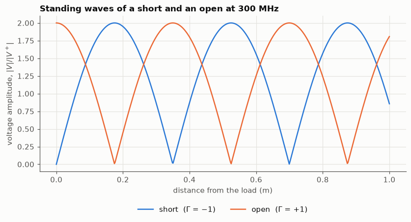
The two patterns have the same shape, shifted by a quarter wavelength (0.175 m). At the load itself the short forces the voltage to zero, while the open has a voltage maximum (and zero current). The first zero of the open is a quarter wavelength in front of it.

A consequence worth remembering: an open circuit seen through a quarter wavelength of line looks like a short, and the other way round.

3. From return loss to impedance

Return loss \(= -20\log_{10}|\Gamma|\), so \(|\Gamma| = 10^{-RL/20}\). For a purely resistive load, \(\Gamma = \pm|\Gamma|\), and \(R = Z_0 (1 + \Gamma)/(1 - \Gamma)\).

return_loss_db = 10.0
gamma_max = 10 ** (-return_loss_db / 20)
r_low = z0 * (1 - gamma_max) / (1 + gamma_max)
r_high = z0 * (1 + gamma_max) / (1 - gamma_max)

print(f"Largest |Γ| allowed:       {gamma_max:.3f}")
print(f"Power reflected, at most:  {gamma_max**2:.0%}")
print(f"Resistive impedance range: {r_low:.1f} Ω to {r_high:.1f} Ω")

Largest |Γ| allowed:       0.316
Power reflected, at most:  10%
Resistive impedance range: 26.0 Ω to 96.2 Ω

A return loss of 10 dB allows \(|\Gamma|\) up to 0.316: 10 % of the power reflected, 90 % delivered. If the impedance is purely resistive it lies between 26 Ω and 96 Ω. The two limits are \(Z_0/1.92\) and \(1.92\,Z_0\): the specification is symmetric as a ratio to 50 Ω, not as a difference. “Better than 10 dB” is a loose requirement, which is why it is so common in antenna datasheets.

4. A longer cable

With a longer cable the reflected wave accumulates phase faster with frequency.

f_hz = np.linspace(50e3, 1.45e9, 401)

fig, ax = plt.subplots()
for length in (0.20, 1.0):
    tau = length / v
    s11 = reflection(75.0) * np.exp(-4j * np.pi * f_hz * tau)
    phase = np.unwrap(np.angle(s11))
    ax.plot(f_hz / 1e6, np.degrees(phase), label=f"{length:g} m of cable")

    slope = np.polyfit(f_hz, phase, 1)[0]  # rad per Hz
    tau_estimated = -slope / (4 * np.pi)
    print(
        f"{length:g} m: delay from the phase slope {tau_estimated * 1e9:.2f} ns, "
        f"length / v = {tau * 1e9:.2f} ns"
    )
ax.set(xlabel="frequency (MHz)", ylabel="unwrapped phase of $S_{11}$ (°)")
ax.set_title("Phase of the reflection for two cable lengths")
ax.legend(loc="lower left");

0.2 m: delay from the phase slope 0.95 ns, length / v = 0.95 ns
1 m: delay from the phase slope 4.77 ns, length / v = 4.77 ns

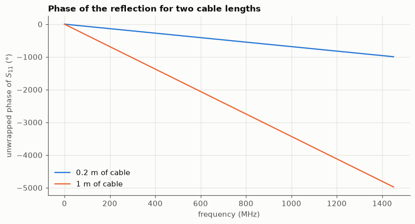
The phase is a straight line whose slope is proportional to the cable length: five times longer, five times steeper. From \(\angle S_{11} = -4\pi f\tau\), the one-way delay is \(\tau = -\text{slope}/(4\pi)\), and it matches \(\ell/v\) exactly.

Two practical notes. np.unwrap removes the ±180° jumps, but only if the phase changes by less than 180° between neighbouring points: a long cable needs a dense frequency grid. And this is exactly the method used on real data in notebook 03 to find the line hidden in front of a resistor.