02 · Systematic errors: the three-term model

A vector network analyzer never shows you the reflection coefficient of your device. It shows you that reflection coefficient after it has gone through the instrument’s own imperfections. In this notebook you build an imperfect instrument yourself, one flaw at a time, and watch what each flaw does to a device you know.

Learning objectives

After this notebook you will be able to:

• name the three systematic error terms of a one-port measurement (directivity, source match and reflection tracking) and say where each one comes from;

• write the equation that links the true reflection coefficient \(\Gamma\) to the measured one \(\Gamma_m\);

• predict which devices each error term distorts most;

• recognise in real data that a raw measurement cannot be trusted.

You need: the relation between impedance and reflection coefficient, \(\Gamma = (Z - Z_0)/(Z + Z_0)\), from notebook 01. No hardware.

import sys

if "google.colab" in sys.modules:
    %pip install -q git+https://github.com/telmomm/nanovna-measurement-course

import matplotlib.pyplot as plt
import numpy as np

from vnacourse import plotting
from vnacourse.data import load_repetitions
from vnacourse.errormodel import ErrorTerms, synthetic_error_terms
from vnacourse.reflection import gamma_to_z, z_to_gamma

plotting.use_course_style()

1. Three ways an instrument distorts a reflection

To measure a reflection, the instrument sends a wave to the device under test (DUT), separates the wave that comes back, and divides one by the other. Three things go wrong on the way:

• Directivity, \(e_{00}\). The part that separates the returning wave (a bridge or a directional coupler) is not perfect: a little of the sent wave leaks straight into the receiver without ever reaching the DUT. The instrument sees a reflection even when there is none.

• Source match, \(e_{11}\). The test port is not exactly 50 Ω. Part of the wave reflected by the DUT bounces off the port and travels to the DUT again, and again.

• Reflection tracking, \(e_{10}e_{01}\). The path to the DUT and back (cables, connectors, receivers) attenuates and delays the wave, differently at each frequency.

These errors are called systematic because they are the same every time you repeat the measurement. That is what makes them removable. Noise and a connector tightened differently each time are random errors; calibration does not remove those.

The figure below is the standard picture of the model: a perfect instrument on the left, the DUT on the right, and in between an “error adapter” that holds the three terms. Follow the arrows from sent to received.

plotting.draw_error_adapter();

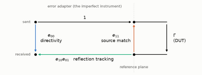
There are two ways to get from sent to received:

1. straight down through \(e_{00}\), never touching the DUT;

2. across to the DUT, reflect (\(\Gamma\)), and back through \(e_{10}e_{01}\). On the way, the wave can also take the loop DUT → \(e_{11}\) → DUT any number of times, which multiplies the path by \(1 + e_{11}\Gamma + (e_{11}\Gamma)^2 + \dots = 1/(1 - e_{11}\Gamma)\).

Adding both paths gives the three-term error model:

\[\Gamma_m = e_{00} + \frac{e_{10}e_{01}\,\Gamma}{1 - e_{11}\,\Gamma}\]

All four quantities are complex numbers, and the three error terms change with frequency. A perfect instrument has \(e_{00} = 0\), \(e_{11} = 0\) and \(e_{10}e_{01} = 1\), and then \(\Gamma_m = \Gamma\).

2. Build your own imperfect instrument

The model is one line of code. terms holds the three error terms in the order (directivity, source match, tracking).

def apply_error_model(gamma, terms):
    """What an imperfect instrument reports for a true reflection `gamma`."""
    e00, e11, tracking = terms
    return e00 + tracking * gamma / (1 - e11 * gamma)


perfect = ErrorTerms(directivity=0, source_match=0, tracking=1)
print(apply_error_model(0.2, perfect))

0.2

We test the instrument with four devices whose true reflection coefficient we know exactly:

Device	Impedance	True \(\Gamma\)
short	0 Ω	−1
open	∞	+1
load	50 Ω	0
resistor	75 Ω	+0.2

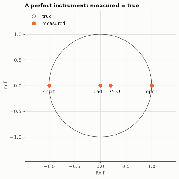
The helper below plots, for each device, where it really is on the \(\Gamma\) plane and where the instrument says it is.

devices = {
    "short": -1.0,
    "open": 1.0,
    "load": 0.0,
    "75 Ω": float(z_to_gamma(75).real),
}


def compare(terms, title):
    """Plot true and measured reflection coefficient of the four test devices."""
    fig, ax = plt.subplots(figsize=(5.2, 5.2))
    plotting.gamma_plane(ax, radius=1.4, title=title)
    # The load and the 75 Ω resistor are close together: push their labels apart.
    offsets = {"load": (4, -16), "75 Ω": (-4, -16)}
    aligns = {"load": "right", "75 Ω": "left"}
    for name, gamma in devices.items():
        measured = apply_error_model(gamma, terms)
        ax.annotate(
            "",
            xy=(measured.real, measured.imag),
            xytext=(gamma, 0),
            arrowprops={"arrowstyle": "-", "color": plotting.INK_SECONDARY, "linewidth": 0.8},
        )
        ax.plot(gamma, 0, "o", color=plotting.SERIES[0], markerfacecolor=plotting.SURFACE)
        ax.plot(measured.real, measured.imag, "o", color=plotting.SERIES[1])
        ax.annotate(
            name,
            (gamma, 0),
            xytext=offsets.get(name, (0, -16)),
            textcoords="offset points",
            ha=aligns.get(name, "center"),
        )
    ax.plot([], [], "o", color=plotting.SERIES[0], markerfacecolor=plotting.SURFACE, label="true")
    ax.plot([], [], "o", color=plotting.SERIES[1], label="measured")
    ax.legend(loc="upper left")
    return ax


compare(perfect, "A perfect instrument: measured = true");

2.1 Directivity only

Give the instrument a single flaw: a directivity of magnitude 0.15.

Predict before you run. The 50 Ω load reflects nothing. What will this instrument report for it? Will the four devices move by the same amount, or by different amounts?

only_directivity = ErrorTerms(directivity=0.15 * np.exp(1j * np.pi / 3), source_match=0, tracking=1)
compare(only_directivity, "Directivity only: everything shifts");

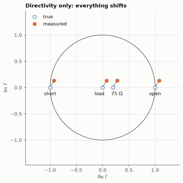
Every device moves by the same vector, \(e_{00}\). The absolute error is the same for all, but the relative error is not: the short and the open (magnitude 1) barely notice, while the load, which should read exactly 0, now reads 0.15. Directivity limits how small a reflection you can measure. It is the term that matters when you want to know how well matched something is.

2.2 Reflection tracking only

Now the only flaw is the return path: it loses 20 % of the amplitude and adds 40° of phase delay.

Predict before you run. Which device will not move at all?

only_tracking = ErrorTerms(
    directivity=0, source_match=0, tracking=0.8 * np.exp(-1j * np.radians(40))
)
compare(only_tracking, "Tracking only: everything scales and rotates");

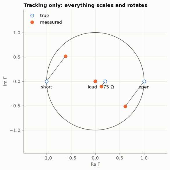
Tracking multiplies \(\Gamma\): the whole plane shrinks and rotates around the centre. The load sits at the centre, so it does not move. The devices far from the centre move the most. If the tracking magnitude is above 1, a short or an open will read as \(|\Gamma_m| > 1\), as if the device reflected more than it received. Keep that in mind for section 4.

2.3 Source match only

Last flaw on its own: a test port that is not 50 Ω, with \(|e_{11}| = 0.25\).

Predict before you run. Look at the equation. For which device does \(e_{11}\) drop out completely? And is the error of the short the same as the error of the open?

only_match = ErrorTerms(directivity=0, source_match=0.25 * np.exp(1j * np.pi / 4), tracking=1)
compare(only_match, "Source match only: the error depends on the device");

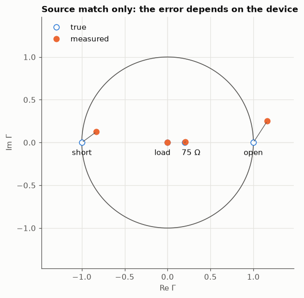
Source match only acts through the product \(e_{11}\Gamma\), so it needs a reflection to exist: the load is untouched, the 75 Ω resistor moves a little, and the short and the open move a lot, each in a different direction. This is the term that makes the error model non-linear in \(\Gamma\), and the reason a simple “subtract and divide” correction is not enough.

Term	Effect on the \(\Gamma\) plane	Hurts most
Directivity \(e_{00}\)	shifts every point by the same vector	small reflections (well-matched devices)
Tracking \(e_{10}e_{01}\)	scales and rotates around the centre	large reflections
Source match \(e_{11}\)	bends the plane; error grows with \(\lvert\Gamma\rvert\)	large reflections

3. All three at once, across frequency

A real instrument has the three flaws together, and each of them changes with frequency. The course package provides a made-up instrument, synthetic_error_terms, with exaggerated errors so that everything is visible. We sweep it from 50 kHz to 1.45 GHz, the same band as the real measurements you will use later.

f_hz = np.linspace(50e3, 1.45e9, 401)
f_mhz = f_hz / 1e6
terms = synthetic_error_terms(f_hz)

fig, ax = plt.subplots()
ax.plot(f_mhz, np.abs(terms.directivity), label="directivity $|e_{00}|$")
ax.plot(f_mhz, np.abs(terms.source_match), label="source match $|e_{11}|$")
ax.plot(f_mhz, np.abs(terms.tracking), label="tracking $|e_{10}e_{01}|$")
ax.set(xlabel="frequency (MHz)", ylabel="magnitude", ylim=(0, 1.05))
ax.set_title("Error terms of the synthetic instrument")
ax.legend(loc="center right");

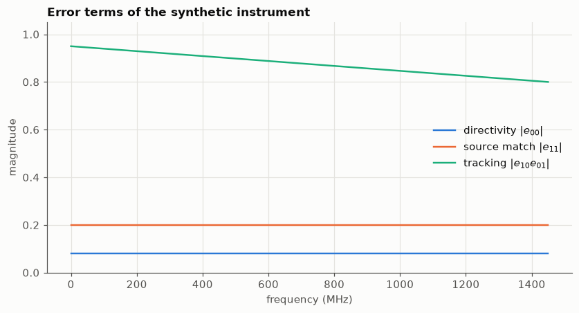
The magnitudes are smooth, almost flat lines. The phases, not shown, rotate with frequency because every path inside the instrument has some length.

Connect the 75 Ω resistor. Its true reflection coefficient is 0.2 at every frequency: a flat line.

Predict before you run. The error terms are smooth. Will the measured \(|\Gamma_m|\) be a smooth, slightly shifted line too?

gamma_true = np.full(f_hz.shape, z_to_gamma(75))
gamma_measured = apply_error_model(gamma_true, terms)

fig, ax = plt.subplots()
ax.plot(f_mhz, np.abs(gamma_true), label="true")
ax.plot(f_mhz, np.abs(gamma_measured), label="measured")
ax.set(xlabel="frequency (MHz)", ylabel="$|\\Gamma|$", ylim=(0, 0.35))
ax.set_title("75 Ω resistor seen by the synthetic instrument")
ax.legend(loc="lower right");

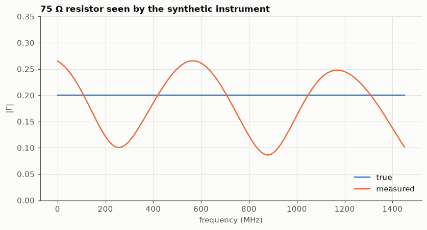
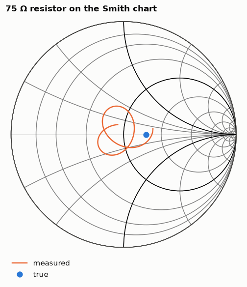
The measured trace has a ripple that is in neither the device nor the magnitudes of the error terms. It comes from the phases. \(\Gamma_m\) is a sum of complex vectors, and as frequency changes they rotate at different rates: where they line up the reading is high, where they oppose each other it is low. Ripple on a trace that should be flat is the classic signature of an uncalibrated (or badly calibrated) measurement.

On the \(\Gamma\) plane the true device is a single point, and the measurement wanders around it:

fig, ax = plt.subplots(figsize=(5.2, 5.2))
plotting.gamma_plane(ax, title="75 Ω resistor on the Smith chart")
ax.plot(gamma_measured.real, gamma_measured.imag, color=plotting.SERIES[1], label="measured")
ax.plot(gamma_true[0].real, gamma_true[0].imag, "o", color=plotting.SERIES[0], label="true")
ax.legend(loc="upper left", bbox_to_anchor=(0.0, 0.0));

What you usually want is not \(\Gamma\) but the impedance. Convert both traces:

z_measured = gamma_to_z(gamma_measured)

fig, ax = plt.subplots()
ax.plot(f_mhz, gamma_to_z(gamma_true).real, label="true")
ax.plot(f_mhz, z_measured.real, label="measured")
ax.set(xlabel="frequency (MHz)", ylabel="resistance, Re Z (Ω)")
ax.set_title("Resistance of the 75 Ω resistor according to the instrument")
ax.legend(loc="upper right")

print(f"Apparent resistance: {z_measured.real.min():.0f} Ω to {z_measured.real.max():.0f} Ω")
print(f"Apparent reactance:  {z_measured.imag.min():.0f} Ω to {z_measured.imag.max():.0f} Ω")

Apparent resistance: 31 Ω to 85 Ω
Apparent reactance:  -15 Ω to 22 Ω

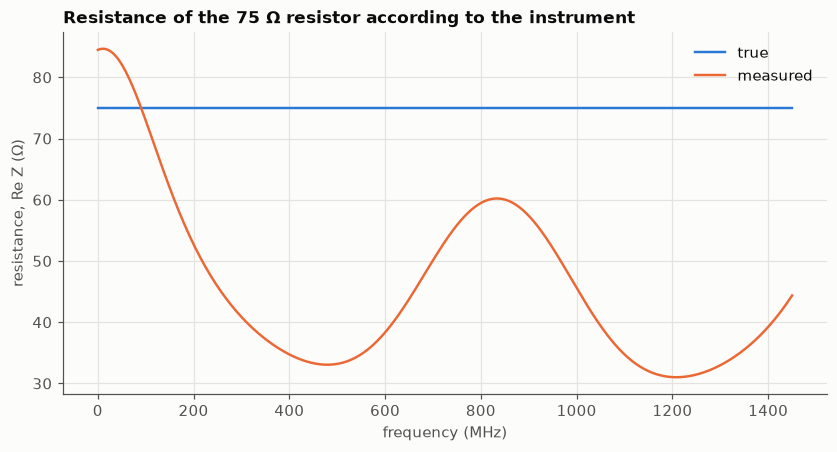
A plain resistor appears to change its resistance with frequency and to have a reactance that it does not have. Nothing here is noise: run the cell again and you get exactly the same wrong answer. An uncalibrated instrument is not imprecise, it is consistently wrong.

The function you wrote is also available as vnacourse.errormodel.apply_error_model, so the next notebook can reuse it. Check that both agree:

from vnacourse import errormodel

assert np.allclose(gamma_measured, errormodel.apply_error_model(gamma_true, terms))
print("Same result as vnacourse.errormodel.apply_error_model")

Same result as vnacourse.errormodel.apply_error_model

4. A real instrument

So far everything was simulated. The repository includes real measurements taken with a NanoVNA-F V2: an open, a short and a 50 Ω load, each measured ten times, saved as the instrument reported them. See data/README.md for the details.

load_repetitions returns the frequency axis and one row per repetition. We average the ten repetitions of each standard.

Predict before you run. If the instrument were perfect, what would \(|\Gamma_m|\) be for the open, the short and the load?

f_real, open_raw = load_repetitions("standards", "open")
_, short_raw = load_repetitions("standards", "short")
_, load_raw = load_repetitions("standards", "load")
print(f"{open_raw.shape[0]} repetitions, {open_raw.shape[1]} frequency points")
print(f"from {f_real[0] / 1e3:.0f} kHz to {f_real[-1] / 1e9:.2f} GHz")

fig, ax = plt.subplots()
ax.plot(f_real / 1e6, np.abs(open_raw.mean(axis=0)), label="open")
ax.plot(f_real / 1e6, np.abs(short_raw.mean(axis=0)), label="short")
ax.plot(f_real / 1e6, np.abs(load_raw.mean(axis=0)), label="load")
ax.axhline(1, color=plotting.INK_SECONDARY, linewidth=0.8, linestyle="--")
ax.set(xlabel="frequency (MHz)", ylabel="$|\\Gamma_m|$")
ax.set_title("Raw readings of the three standards (NanoVNA-F V2)")
ax.legend(loc="upper right")

print(f"Largest raw |Γm| of the open: {np.abs(open_raw.mean(axis=0)).max():.2f}")

10 repetitions, 1001 frequency points
from 50 kHz to 1.45 GHz
Largest raw |Γm| of the open: 2.13

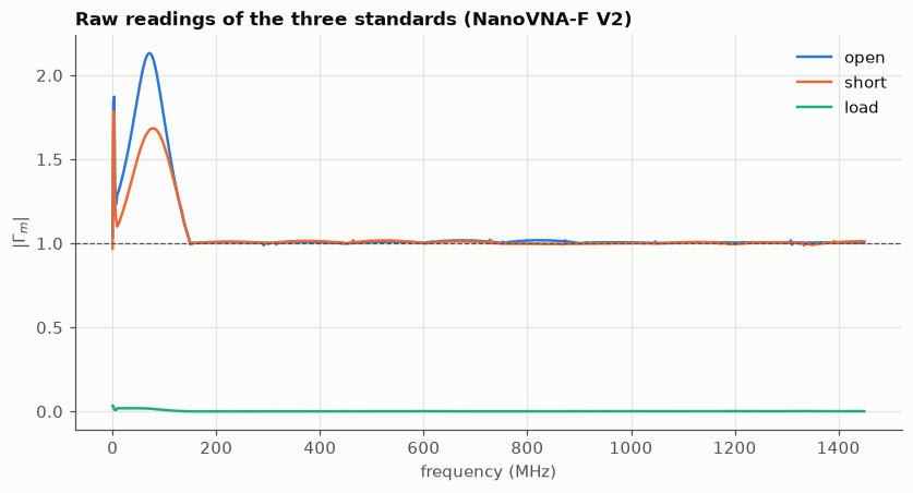
Below about 150 MHz the open and the short read well above 1: according to the instrument they send back up to twice the wave they receive. An open circuit and a short circuit are passive, so they cannot do that. The only explanation is the instrument, and section 2.2 told you which term produces this.

Above 150 MHz the three traces look almost ideal. “Almost” is the important word: how far from ideal they are, and how to remove what is left, is the subject of the next notebook.

Check your understanding

1. An instrument has \(e_{00} = 0.05\) and is otherwise perfect. You measure an antenna and read \(|\Gamma_m| = 0.05\). What can you say about the true \(|\Gamma|\) of the antenna?

Answer

Only that it lies between 0 and 0.10. The reading is the sum of the true reflection and the directivity, and you do not know their relative phase: they may add, or cancel. When the reading is as small as the directivity, the measurement tells you almost nothing.

2. Why does the 50 Ω load not move in sections 2.2 and 2.3?

Answer

Tracking and source match both multiply \(\Gamma\) in the model. With \(\Gamma = 0\) nothing comes back from the DUT, so there is nothing to scale and nothing to re-reflect. Only directivity, which does not involve the DUT, is left: for a perfect load, \(\Gamma_m = e_{00}\).

3. You measure the same device five times in a row without touching anything and the five traces overlap perfectly. Does that mean the measurement is accurate?

Answer

No. It means the measurement is repeatable: random errors are small. Systematic errors are identical in the five traces, so they are invisible in this test.

Exercises

Worked solutions are in exercises/solutions/02_solutions.ipynb.

1. Which term is to blame? Using the synthetic instrument of section 3, switch the terms off one at a time (set directivity or source match to 0, or tracking to 1) and plot the measured \(|\Gamma_m|\) of the 75 Ω resistor each time. Which term contributes most to the ripple? Does the answer change if the device is a short?

2. Ripple and length. In synthetic_error_terms the phase of each term rotates because of a delay. Build your own ErrorTerms where the source match is \(0.2\,e^{-j 2\pi f \tau}\) and try \(\tau\) = 0.5 ns, 1 ns and 2 ns with a short as the device. How does the spacing between ripple peaks depend on \(\tau\)? What does that tell you about a ripple you see on a real instrument with a long cable?

3. Worst case. For an instrument with \(|e_{00}| = 0.03\) and no other error, compute the range of readings you could get for a device with true \(|\Gamma| = 0.1\). Express both ends as return loss, \(-20\log_{10}|\Gamma|\), in dB.

4. Real data. Plot the phase of the raw open and of the raw short from section 4. Ideally they should be 0° and 180° at every frequency. Are they? Plot the ten repetitions of the open on top of each other: can you see any difference between them?

# Your work here

Summary

• A one-port measurement is distorted by three systematic error terms: directivity \(e_{00}\), source match \(e_{11}\) and reflection tracking \(e_{10}e_{01}\).

• They combine as \(\Gamma_m = e_{00} + \dfrac{e_{10}e_{01}\,\Gamma}{1 - e_{11}\,\Gamma}\).

• Directivity hurts small reflections; tracking and source match hurt large ones.

• Because the terms are complex and rotate with frequency, they produce ripple and false reactance, even on a plain resistor.

• Systematic errors repeat exactly. That is bad news (repeating the measurement does not help) and good news: three unknowns per frequency can be solved for.

Next: in 03 · SOL calibration you measure three known devices, solve for the three error terms and undo the distortion, first on this synthetic instrument and then on the real data.