

Solutions · 05 Validation and measurement quality#
Worked solutions to the exercises of notebook 05. Try each exercise yourself first.
import sys

if "google.colab" in sys.modules:
    %pip install -q "vnacourse[validation] @ git+https://github.com/telmomm/nanovna-measurement-course"
import matplotlib.pyplot as plt
import numpy as np
import skrf as rf
from numpy.lib.stride_tricks import sliding_window_view
from rfmeasurement.domain import (
    Measurement,
    MeasurementContext,
    MetadataConfidence,
    ValidationResult,
    ValidationStatus,
)
from rfmeasurement.validation import ValidationRule

from vnacourse import calibration, plotting
from vnacourse.data import load_repetitions

plotting.use_course_style()

f_hz, short_reps = load_repetitions("standards", "short")
_, open_reps = load_repetitions("standards", "open")
_, load_reps = load_repetitions("standards", "load")
_, resistor_reps = load_repetitions("dut", "load_75ohm")
f_mhz = f_hz / 1e6
standards = (short_reps, open_reps, load_reps)
1. Mean or median?#
The median of complex numbers is taken on the real and imaginary parts separately. Everything else is as in section 4: calibrate with repetitions 1–5, test on repetitions 6–10 of the open.
def mean(repetitions):
    return repetitions.mean(axis=0)


def median(repetitions):
    return np.median(repetitions.real, axis=0) + 1j * np.median(repetitions.imag, axis=0)


fig, ax = plt.subplots()
for name, combine in (("mean", mean), ("median", median)):
    terms = calibration.solve_error_terms([combine(reps[:5]) for reps in standards])
    distance = np.abs(calibration.correct(combine(open_reps[5:]), terms) - 1)
    ax.semilogy(f_mhz, distance, label=name, linewidth=1.0)
    print(
        f"{name:<7} typical {np.median(distance):.4f}   worst {distance.max():.4f}   "
        f"points beyond 0.01: {np.sum(distance > 0.01)}"
    )
ax.set(xlabel="frequency (MHz)", ylabel="$|\\Gamma - 1|$ of the calibrated open (log scale)")
ax.set_title("Combining repetitions with the mean or with the median")
ax.legend(loc="upper center", bbox_to_anchor=(0.5, -0.18), ncol=2);
mean    typical 0.0016   worst 0.0404   points beyond 0.01: 42
median  typical 0.0013   worst 0.0190   points beyond 0.01: 6
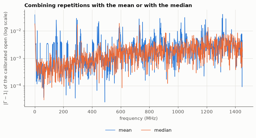
The median wins clearly on the spikes: the worst point drops from 0.040 to 0.019 and the number of points further than 0.01 from the ideal value falls from 42 to 6. The typical distance improves slightly too.
The mean of five values is pulled by one bad value by a fifth of its size; the median ignores it as long as fewer than half the values are bad. The price: for clean, normally distributed noise the median is a little noisier than the mean. When the data has outliers, as here, it is a good trade. Better still is to find out why the spikes occur and avoid them at acquisition.
2. Uncertainty across the band#
Ten calibrations, one per repetition of the standards, each applied to the mean sweep of the resistor. Their scatter at each frequency is the contribution of the calibration’s repeatability to the corrected \(\Gamma\).
resistor_mean = resistor_reps.mean(axis=0)
corrected = np.array(
    [
        calibration.correct(
            resistor_mean,
            calibration.solve_error_terms([short_reps[i], open_reps[i], load_reps[i]]),
        )
        for i in range(len(open_reps))
    ]
)
scatter = np.sqrt(corrected.real.var(axis=0, ddof=1) + corrected.imag.var(axis=0, ddof=1))

fig, ax = plt.subplots()
ax.semilogy(f_mhz, scatter, linewidth=1.0)
ax.set(xlabel="frequency (MHz)", ylabel="standard deviation of corrected Γ (log scale)")
ax.set_title("75 Ω resistor: scatter across ten calibrations")

for label, band in (
    ("below 150 MHz", f_hz < 150e6),
    ("150 to 500 MHz", (f_hz >= 150e6) & (f_hz < 500e6)),
    ("above 1 GHz", f_hz > 1e9),
):
    print(f"{label:<15} typical scatter {np.median(scatter[band]):.5f}")
print(f"worst point: {scatter.max():.4f} at {f_mhz[scatter.argmax()]:.2f} MHz")
below 150 MHz   typical scatter 0.00074
150 to 500 MHz  typical scatter 0.00053
above 1 GHz     typical scatter 0.00096
worst point: 0.0100 at 0.05 MHz
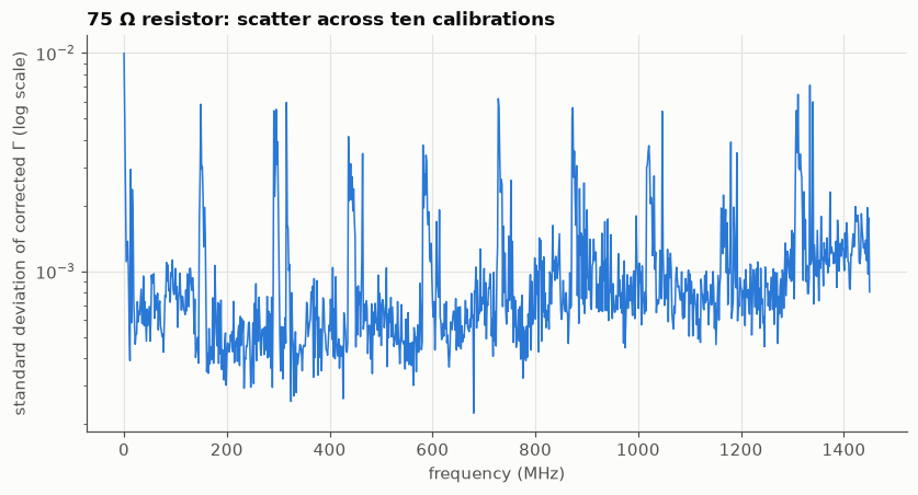
Not uniform. The calibration repeats best between 150 MHz and 500 MHz (about 0.0005), is roughly twice as noisy above 1 GHz, and is also worse below 150 MHz, the band where the instrument’s raw response is far from ideal. The spikes of section 2 carry over into the calibrated result, and the very first point of the sweep is the worst.
Compare the level with section 2: the standards scatter by about 0.003, but the corrected resistor only by about 0.0007. The scatter of the short and the open enters the result multiplied by the resistor’s small \(|\Gamma| = 0.2\); a device near the rim of the chart would inherit it in full. The uncertainty of a calibrated result depends on the device as well as on the calibration.
3. Write a rule#
A spike is a point that departs from its neighbours. Compare each point of \(|\Gamma|\) with the median of a window of seven points centred on it; the median follows the smooth trend and ignores a single outlier.
class SpikesRule(ValidationRule):
    """Warn when points depart from the local median of |Γ| by more than a threshold."""

    identifier = "quality.spikes"
    description = "No point departs from the median of its neighbours by more than the threshold."

    def __init__(self, threshold=0.02, window=7):
        self.threshold = threshold
        self.window = window

    def _evaluate(self, measurement):
        magnitude = np.abs(measurement.data.s[:, 0, 0])
        padded = np.pad(magnitude, self.window // 2, mode="edge")
        local_median = np.median(sliding_window_view(padded, self.window), axis=1)
        spikes = np.flatnonzero(np.abs(magnitude - local_median) > self.threshold)
        return ValidationResult(
            rule_id=self.identifier,
            status=ValidationStatus.WARNING if len(spikes) else ValidationStatus.PASS,
            description=self.description,
            evidence={
                "threshold": self.threshold,
                "n_spikes": len(spikes),
                "frequency_indices": spikes.tolist(),
            },
            explanation="Isolated departures from the local trend." if len(spikes) else None,
        )


frequency = rf.Frequency.from_f(f_hz, unit="Hz")
rule = SpikesRule()
for repetition in (0, 8):
    sweep = Measurement(
        data=rf.Network(frequency=frequency, s=open_reps[repetition], z0=50),
        context=MeasurementContext(dut="open", instrument="NanoVNA-F V2", calibration="none (raw)"),
    )
    result = rule.evaluate(sweep)
    indices = result.evidence["frequency_indices"]
    print(f"repetition {repetition + 1}: {result.status.value}, spikes at points {indices}")
    print("   frequencies (MHz):", np.round(f_mhz[indices], 1))
repetition 1: warning, spikes at points [1, 2, 3, 4, 5]
   frequencies (MHz): [1.5 2.9 4.4 5.8 7.3]
repetition 9: warning, spikes at points [1, 2, 3, 4, 5, 301, 502, 904]
   frequencies (MHz): [   1.5    2.9    4.4    5.8    7.3  436.5  727.9 1310.8]
The rule finds three genuine spikes in repetition 9, at points 301, 502 and 904: all just after a multiple of 100, as section 2 found from the statistics of ten sweeps. Here a single sweep is enough.
It also flags points 1 to 5 in both repetitions. Those are not spikes. At the very bottom of the band the raw response of this instrument really does change abruptly from one point to the next, and a rule that looks for “departure from the neighbours” cannot tell a fast real change from an outlier. This is why the rule returns a warning with its evidence, not a fail: it points at places to look, and a person decides what they are. A rule tuned until it never raised a false alarm on this dataset would be a rule fitted to this dataset.
4. Your own context#
There is no single right answer. Here is one for an imagined measurement of a skin electrode, with the reasoning for each confidence level.
context = MeasurementContext(
    dut="Ag/AgCl electrode, batch 12, sample 3",
    operator="A. Student",
    instrument="NanoVNA-F V2, serial 0421",
    calibration="SOL at the end of the test cable, kit definitions from the supplier",
    cables="30 cm RG-316, SMA",
    fixture="custom electrode holder, revision B",
    temperature_c=23.5,
    averaging=10,
    frequency_range_hz=(50e3, 1.45e9),
    confidence={
        "dut": MetadataConfidence.SPECIFIED,
        "instrument": MetadataConfidence.SPECIFIED,
        "calibration": MetadataConfidence.SPECIFIED,
        "cables": MetadataConfidence.SPECIFIED,
        "temperature_c": MetadataConfidence.MEASURED,
        "frequency_range_hz": MetadataConfidence.MEASURED,
        "averaging": MetadataConfidence.MEASURED,
    },
)

for field in context.__dataclass_fields__:
    value = getattr(context, field)
    if field == "confidence":
        continue
    level = context.confidence.get(field)
    print(
        f"{field:<20} {str(value) if value not in (None, {}) else '— unknown':<70} "
        f"{level.value if level else ''}"
    )
dut                  Ag/AgCl electrode, batch 12, sample 3                                  specified
operator             A. Student
instrument           NanoVNA-F V2, serial 0421                                              specified
calibration          SOL at the end of the test cable, kit definitions from the supplier    specified
cables               30 cm RG-316, SMA                                                      specified
fixture              custom electrode holder, revision B
temperature_c        23.5                                                                   measured
humidity_percent     — unknown
pressure_pa          — unknown
rf_power_dbm         — unknown
if_bandwidth_hz      — unknown
averaging            10                                                                     measured
sweep_settings       — unknown
frequency_range_hz   (50000.0, 1450000000.0)                                                measured
timestamp            — unknown
Measured: what an instrument read during the session (temperature from a thermometer on the bench, the frequency range and averaging from the sweep itself).
Specified: what you were told and wrote down (the part’s label, the instrument’s serial number, the kit definitions from the supplier). You trust a document, not a reading.
Estimated or assumed: anything you did not check. If you had not measured the temperature and wrote “about 23 °C because the laboratory is air-conditioned”, that is assumed, and saying so is more useful than a bare number.
Unknown: left empty. Humidity, pressure, RF power and IF bandwidth are empty here; an empty field is an honest answer, a guessed one is not.
The fields that most often turn out to matter later, and are most often missing, are the calibration (where and with what), the cables and fixture, and the date.