00 · What does a VNA measure?

You already know how to measure a voltage with a multimeter and how to look at a signal on an oscilloscope. A vector network analyzer (VNA) answers a different question: when I send a wave into this device, how much comes back, and with what delay? This notebook explains why that is the right question at radio frequency, and what the answer looks like.

Learning objectives

After this notebook you will be able to:

• explain what the incident and reflected waves at a port are, and why they appear;

• define the S-parameters of a one-port and a two-port network;

• compute how much power a load reflects, and express it as return loss;

• tell what a VNA measures that a multimeter or an oscilloscope does not.

You need: phasors and complex impedance, and basic NumPy and Matplotlib. No hardware.

import sys

if "google.colab" in sys.modules:
    %pip install -q git+https://github.com/telmomm/nanovna-measurement-course

import matplotlib
import matplotlib.pyplot as plt
import numpy as np
import skrf as rf

import vnacourse
from vnacourse import plotting

plotting.use_course_style()

for module in (np, matplotlib, rf, vnacourse):
    print(f"{module.__name__:<12} {module.__version__}")

numpy        2.5.3
matplotlib   3.11.2
skrf         2.1.0
vnacourse    0.9.0

If the cell above printed four version numbers, your environment is ready for the whole course.

1. When a wire stops being a wire

In circuit theory a wire is a node: the voltage is the same at both ends, at every instant. That is an approximation. A signal travels along a cable at a finite speed \(v\), about 70 % of the speed of light in a typical coaxial cable, so a sinusoid of frequency \(f\) occupies a length

\[\lambda = \frac{v}{f}\]

along the cable. If the cable is much shorter than this wavelength, both ends see practically the same voltage and the approximation holds. If it is not, the voltage depends on where along the cable you look.

Predict before you run. You have a 1 m cable. At which of these frequencies does it stop being “just a wire”: 50 Hz, 1 MHz, 100 MHz, 1 GHz?

c0 = 299_792_458.0  # speed of light in vacuum, m/s
v = 0.7 * c0  # wave speed in a typical coaxial cable
cable_length = 1.0  # m

print(f"{'frequency':>10}  {'wavelength':>12}  {'1 m cable, in wavelengths':>26}")
for f in (50, 1e3, 1e6, 100e6, 1e9):
    wavelength = v / f
    print(f"{f:10.3g}  {wavelength:10.3g} m  {cable_length / wavelength:26.2g}")

 frequency    wavelength   1 m cable, in wavelengths
        50     4.2e+06 m                     2.4e-07
     1e+03     2.1e+05 m                     4.8e-06
     1e+06         210 m                      0.0048
     1e+08         2.1 m                        0.48
     1e+09        0.21 m                         4.8

At 50 Hz the wavelength is thousands of kilometres and the cable is nothing. At 1 MHz it is still less than a hundredth of a wavelength. At 100 MHz the cable is half a wavelength long, and at 1 GHz it holds almost five. A common rule of thumb: once a connection is longer than about a tenth of a wavelength, you must think in terms of waves.

That is the regime of a VNA, and it is also the regime of much of biomedical instrumentation that works with radio frequency: wireless implants, wearable antennas, MRI coils, dielectric measurement of tissue.

2. Two waves on one line

A cable designed to carry waves is a transmission line. It has a characteristic impedance \(Z_0\), almost always 50 Ω in instrumentation: the ratio between voltage and current of a wave travelling along it.

Send a wave down the line towards a load of impedance \(Z_L\). At the load, voltage and current must obey \(V = Z_L I\), but the arriving wave carries them in the ratio \(Z_0\). If \(Z_L \neq Z_0\) the two conditions cannot both hold with a single wave, and a second wave appears, travelling back: the reflected wave. Its size relative to the incident one is the reflection coefficient:

\[\Gamma = \frac{V^-}{V^+} = \frac{Z_L - Z_0}{Z_L + Z_0}\]

On the line, the two waves add. At a distance \(d\) from the load, the amplitude of the total voltage is

\[|V(d)| = |V^+|\;\bigl|1 + \Gamma\, e^{-j 2 \beta d}\bigr| \qquad \beta = \frac{2\pi}{\lambda}\]

The factor \(e^{-j2\beta d}\) is the phase the reflected wave has lost travelling to the load and back.

Predict before you run. We plot the voltage amplitude along 1 m of line at 300 MHz, for three loads: 50 Ω, 150 Ω and a short circuit. For which load is the amplitude the same everywhere? For which is it zero somewhere?

z0 = 50.0


def reflection(z_load):
    """Reflection coefficient of a load on a 50 Ω line."""
    return (z_load - z0) / (z_load + z0)


f = 300e6
beta = 2 * np.pi * f / v
d = np.linspace(0, 1.0, 500)  # distance from the load, m

fig, ax = plt.subplots()
for name, z_load in (("50 Ω", 50.0), ("150 Ω", 150.0), ("short", 0.0)):
    gamma = reflection(z_load)
    amplitude = np.abs(1 + gamma * np.exp(-2j * beta * d))
    ax.plot(d, amplitude, label=f"{name}  (Γ = {gamma:+.1f})")
ax.set(xlabel="distance from the load (m)", ylabel="voltage amplitude, $|V| / |V^+|$")
ax.set_title("Voltage along the line at 300 MHz")
ax.legend(loc="upper center", bbox_to_anchor=(0.5, -0.18), ncol=3)

print(f"Wavelength in the cable at 300 MHz: {v / f:.2f} m")

Wavelength in the cable at 300 MHz: 0.70 m

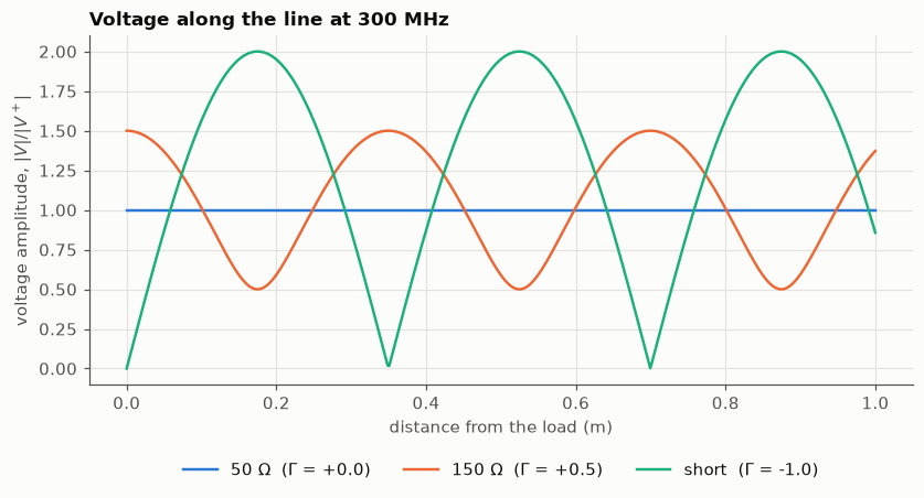
• 50 Ω (\(\Gamma = 0\)): no reflection. The amplitude is the same everywhere. The load is matched.

• 150 Ω (\(\Gamma = +0.5\)): the two waves add in some places and partly cancel in others, giving a standing wave between 0.5 and 1.5.

• Short (\(\Gamma = -1\)): everything is reflected, inverted. The amplitude goes from 0 to twice the incident wave, with zeros every half wavelength.

Imagine probing this line with an oscilloscope. The amplitude you read depends on where you touch, and at every point you see only the sum of the two waves. You cannot tell from one reading how much is going towards the load and how much is coming back.

3. Waves instead of volts: \(a\), \(b\) and \(S_{11}\)

Since the incident and reflected waves are what carries the information, RF engineering works with them directly. At a port, define

\[a = \frac{V^+}{\sqrt{Z_0}} \quad\text{(incident wave)} \qquad b = \frac{V^-}{\sqrt{Z_0}} \quad\text{(reflected wave)}\]

The scaling by \(\sqrt{Z_0}\) makes \(\tfrac12|a|^2\) the power travelling towards the device and \(\tfrac12|b|^2\) the power coming back. Their ratio is the reflection S-parameter:

\[S_{11} = \frac{b_1}{a_1}\]

For a single load at the end of the port, \(S_{11}\) is the reflection coefficient \(\Gamma\). It is a complex number: its magnitude says how much comes back, its phase says with what delay.

Two derived quantities are used all the time:

• the fraction of power reflected, \(|S_{11}|^2\);

• the return loss in decibels, \(-20\log_{10}|S_{11}|\): how far below the incident wave the reflection is. A larger return loss means a better match.

print(f"{'load':>8}  {'Γ':>6}  {'power reflected':>16}  {'return loss':>12}")
for name, z_load in (
    ("short", 0.0),
    ("25 Ω", 25.0),
    ("50 Ω", 50.0),
    ("75 Ω", 75.0),
    ("150 Ω", 150.0),
):
    gamma = reflection(z_load)
    reflected = abs(gamma) ** 2
    return_loss = "∞" if gamma == 0 else f"{abs(20 * np.log10(abs(gamma))):.1f} dB"
    print(f"{name:>8}  {gamma:+6.2f}  {reflected:15.0%}  {return_loss:>12}")
print(f"{'open':>8}  {1:+6.2f}  {1:15.0%}  {'0.0 dB':>12}")

    load       Γ   power reflected   return loss
   short   -1.00             100%        0.0 dB
    25 Ω   -0.33              11%        9.5 dB
    50 Ω   +0.00               0%             ∞
    75 Ω   +0.20               4%       14.0 dB
   150 Ω   +0.50              25%        6.0 dB
    open   +1.00             100%        0.0 dB

A 75 Ω load on a 50 Ω line reflects only 4 % of the power: mismatch is forgiving. Note also that 25 Ω and 100 Ω would give the same \(|\Gamma|\) with opposite signs. The magnitude alone does not tell you which one you have; the phase does.

4. What the VNA does

A VNA has a source that sweeps through a list of frequencies. At each one it sends a wave \(a_1\) out of its port, separates the wave \(b_1\) that comes back, and measures the ratio \(b_1/a_1\) in magnitude and in phase. That last part is the “vector” in the name.

Let us simulate what it would see. The device is a 75 Ω resistor at the end of 20 cm of cable. The cable delays the wave by \(\tau = \ell / v\) each way, so the reflection reaches the port with a phase lag of \(2\pi f \cdot 2\tau\):

\[S_{11}(f) = \Gamma_L\, e^{-j 4\pi f \tau}\]

Predict before you run. The resistor reflects the same fraction of the wave at every frequency. Will anything in \(S_{11}\) change with frequency?

f_hz = np.linspace(50e3, 1.45e9, 401)
f_mhz = f_hz / 1e6

length = 0.20  # m
tau = length / v
a1 = np.ones(f_hz.shape, dtype=complex)  # the incident wave, our reference
b1 = reflection(75.0) * np.exp(-4j * np.pi * f_hz * tau) * a1
s11 = b1 / a1

fig, (ax_mag, ax_phase) = plt.subplots(2, 1, figsize=(7.5, 5.2), sharex=True)
ax_mag.plot(f_mhz, np.abs(a1), label="incident $|a_1|$")
ax_mag.plot(f_mhz, np.abs(b1), label="reflected $|b_1|$")
ax_mag.set(ylabel="magnitude", ylim=(0, 1.2))
ax_mag.set_title("75 Ω resistor behind 20 cm of cable")
ax_mag.legend(loc="center right")
ax_phase.plot(f_mhz, np.degrees(np.angle(s11)), color=plotting.SERIES[2])
ax_phase.set(
    xlabel="frequency (MHz)", ylabel="phase of $S_{11}$ (°)", yticks=[-180, -90, 0, 90, 180]
)

print(f"One-way delay of the cable: {tau * 1e9:.2f} ns")

One-way delay of the cable: 0.95 ns

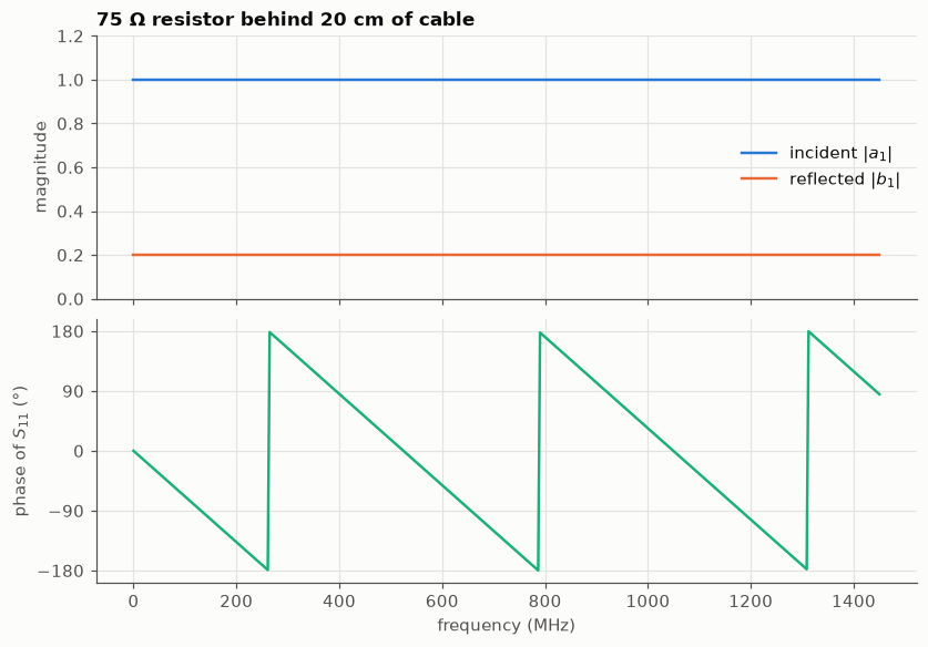
The magnitude is flat at 0.2. The phase falls steadily (the jumps from −180° to +180° are only the angle wrapping around) because the same cable is more wavelengths long at higher frequency. The slope of that phase is a direct measurement of the cable’s delay.

Now look at what an instrument that only measures the total voltage amplitude at the port would report: \(|a_1 + b_1|\).

total = np.abs(a1 + b1)

fig, ax = plt.subplots()
ax.plot(f_mhz, total, color=plotting.SERIES[1])
ax.set(xlabel="frequency (MHz)", ylabel="$|a_1 + b_1|$", ylim=(0, 1.4))
ax.set_title("Total voltage amplitude at the port");

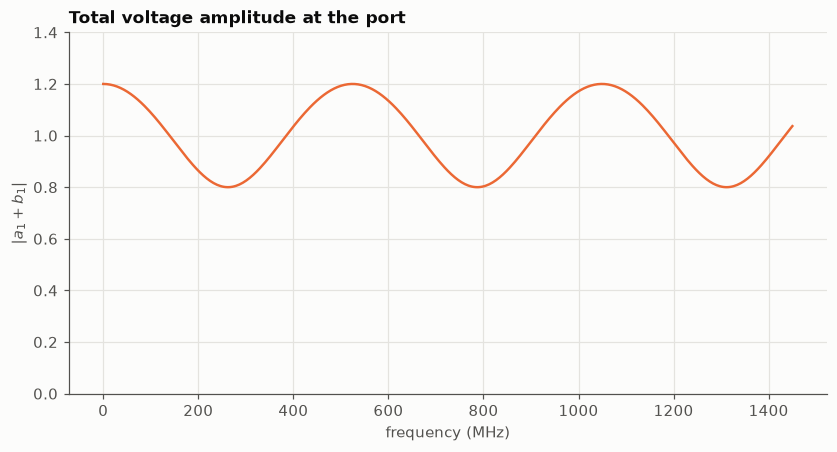
The total voltage swings between 0.8 and 1.2 with frequency. From this curve alone you could not say whether the device changes with frequency or whether you are looking at a constant reflection through a cable. The VNA can, because it keeps the two waves apart and keeps the phase.

The same thing with scikit-rf

scikit-rf is the Python library this course uses to handle S-parameters. Its central object is the Network: a frequency axis plus the S-parameters at each frequency. We build the cable as a two-port network and the resistor as a one-port network, connect them with **, and compare with our formula.

frequency = rf.Frequency.from_f(f_hz, unit="Hz")

s_cable = np.zeros((len(f_hz), 2, 2), dtype=complex)
s_cable[:, 1, 0] = s_cable[:, 0, 1] = np.exp(-2j * np.pi * f_hz * tau)
cable = rf.Network(frequency=frequency, s=s_cable, z0=50, name="20 cm cable")

resistor = rf.Network(
    frequency=frequency, s=np.full(len(f_hz), reflection(75.0)), z0=50, name="75 Ω"
)

device = cable**resistor
device.name = "75 Ω behind 20 cm of cable"
print(device)
print("Same S11 as our formula:", np.allclose(device.s[:, 0, 0], s11))

1-Port Network: '75 Ω behind 20 cm of cable',  50000.0-1450000000.0 Hz, 401 pts, z0=[50.+0.j]
Same S11 as our formula: True

device.s has shape (frequencies, ports, ports), so device.s[:, 0, 0] is \(S_{11}\) at every frequency. You will also meet device.f (frequencies in Hz), device.s_db and device.s_deg.

5. Two ports

The cable above has two ends, so it has two ports and four S-parameters. Each one is “wave out of port \(i\) divided by wave into port \(j\), with the other port matched”:

\[\begin{split} \begin{bmatrix} b_1 \\ b_2 \end{bmatrix} = \begin{bmatrix} S_{11} & S_{12} \\ S_{21} & S_{22} \end{bmatrix} \begin{bmatrix} a_1 \\ a_2 \end{bmatrix} \end{split}\]

• \(S_{11}\), \(S_{22}\): reflection at each port.

• \(S_{21}\), \(S_{12}\): transmission from port 1 to 2 and back.

k = 200  # one frequency point
print(f"S-matrix of the cable at {f_mhz[k]:.0f} MHz:")
print(np.round(cable.s[k], 3))
print(f"|S21| = {abs(cable.s[k, 1, 0]):.2f}, phase {np.degrees(np.angle(cable.s[k, 1, 0])):.0f}°")

S-matrix of the cable at 725 MHz:
[[ 0.   +0.j    -0.362+0.932j]
 [-0.362+0.932j  0.   +0.j   ]]
|S21| = 1.00, phase 111°

Our ideal cable reflects nothing (\(S_{11} = S_{22} = 0\)) and transmits everything (\(|S_{21}| = 1\)) with a phase delay. A filter would have \(|S_{21}| \approx 1\) in its passband and \(\approx 0\) outside; an amplifier would have \(|S_{21}| > 1\).

This course is about one-port measurements: only \(S_{11}\). It is the simplest case, it is what you need to measure an impedance, and all the ideas about error and calibration carry over to two ports.

6. Three instruments

	Multimeter	Oscilloscope	VNA
Measures	voltage, current, resistance	voltage against time, at one point	ratio of waves, against frequency
Stimulus	DC or low frequency	none (it observes)	its own swept sine wave
Result	one number	a waveform	a complex number per frequency
Separates incident from reflected	no	no: it sees their sum	yes
Keeps phase	no	relative to its trigger	yes, relative to its own source
Tells you	“this is 75 Ω” at DC	“the signal looks like this, here”	“this is how the device responds to a wave, at each frequency”

A VNA is the RF counterpart of the ohmmeter: it characterises a device, not a signal. The NanoVNA used in this course is a pocket-sized, low-cost one. As you will see from notebook 02 on, what it reports is not yet the truth about the device.

Check your understanding

1. A load reflects 25 % of the incident power. What is \(|\Gamma|\)? What is the return loss?

Answer

\(|\Gamma| = \sqrt{0.25} = 0.5\). Return loss \(= -20\log_{10} 0.5 = 6\) dB.

2. In section 2, the zeros of the standing wave for the short are 0.35 m apart at 300 MHz. Why that distance?

Answer

The pattern depends on \(e^{-j2\beta d}\), which repeats when \(2\beta d\) grows by \(2\pi\), that is every \(d = \lambda/2\). The wavelength in the cable is 0.70 m, so the zeros are 0.35 m apart.

3. You measure \(|S_{11}| = 0.2\). Can you tell whether the load is 75 Ω or 33 Ω?

Answer

Not from the magnitude: 75 Ω gives \(\Gamma = +0.2\) and 33.3 Ω gives \(\Gamma = -0.2\). The phase (0° or 180°) tells them apart, provided there is no unknown length of cable in front, which would rotate the phase.

4. Why can an oscilloscope not replace a VNA for measuring a reflection?

Answer

At a single point it sees the sum of the incident and reflected waves. Separating them requires either directional hardware (a coupler or bridge, as inside a VNA) or measurements at several known positions.

Exercises

Worked solutions are in exercises/solutions/00_solutions.ipynb. Try them first.

1. How short is short? For a 10 cm cable with \(v = 0.7c\), find the frequency at which it is a tenth of a wavelength long. Repeat for a 1 cm lead of a component. What does this say about measuring at 1 GHz?

2. Open circuit. Add an open circuit (\(Z_L \to \infty\), \(\Gamma = +1\)) to the standing-wave plot of section 2. Where are its zeros compared with those of the short?

3. From return loss to impedance. An antenna datasheet promises a return loss better than 10 dB. What is the largest \(|\Gamma|\) allowed, what fraction of the power may be reflected, and between which two purely resistive values may its impedance lie?

4. A longer cable. In section 4, change the cable from 20 cm to 1 m. How does the phase plot change? Estimate the cable delay from the slope of the unwrapped phase (np.unwrap) and compare it with \(\ell / v\).

# Your work here

Summary

• When a connection is not short compared with the wavelength, voltage depends on position and you must think in waves.

• A load that differs from the line’s \(Z_0\) reflects part of the wave: \(\Gamma = (Z_L - Z_0)/(Z_L + Z_0)\).

• \(S_{11} = b_1/a_1\) is the ratio of reflected to incident wave at a port: a complex number per frequency. \(|S_{11}|^2\) is the fraction of power reflected.

• A VNA generates the incident wave, separates the reflected one, and measures their ratio in magnitude and phase across frequency.

• The phase carries information the magnitude does not: the sign of the mismatch and any delay in front of the device.

Next: 01 · Reflection coefficient and the Smith chart turns \(\Gamma\) into impedance and back, and introduces the chart on which RF engineers read both at once.